Motivation: The 2025 NCAA Women’s Ice Hockey Tournament
The Wisconsin Badgers defeated the Ohio State Buckeyes women in the championship game of the 2025 NCAA Women’s Ice Hockey Tournament1. During the 2024-25 regular season, the Badgers won 38 games, lost 1 game, and tied 2 games. The Buckeyes won 35 games, lost 4 games, and did not tie any games. In this lecture, we’ll consider the broad question “Did the better team win?” and introduce a framework for measuring latent team strength and predicting the outcome of individual matches.
To motivate our developments, let’s consider two slightly different — but certainly related — questions, which are somewhat more nuanced than “did the better team win?”:
If we could repeatedly play the championship game, how often would the Badgers win?
If the NCAA Championship were awarded to the winner in a “best-of-5” series2 at a neutral site, what is the likelihood that the Badgers would win the championship?
To answer these questions, we introduce a model for estimating latent team strengths from pairwise comparisons (i.e., match results; Section 2). We build a data set containing the outcomes of every Division 1 NCAA Women’s Ice Hockey game from the 2024-25 season (Section 3). We then estimate the model parameters (Section 4) before using the model estimates to simulate a best-of-5 series (Section 4.3) between the Badgers and Buckeyes.
The Bradley-Terry Model
Suppose we observe the outcome of \(n\) games played between \(p\) teams, which we label \(1, 2, \ldots, p.\) The basic Bradley-Terry model associates each team \(j = 1, \ldots, p,\) with a latent strength \(\lambda_{j}\) and asserts that \[
\mathbb{P}(\textrm{team i beats team j}) = \frac{e^{\lambda_{i}}}{e^{\lambda_{i}} + e^{\lambda_{j}}} = \frac{1}{1 + e^{-1 \times (\lambda_{i} - \lambda_{j})}}
\] In other words, under the basic Bradley-Terry model, the log-odds of team \(i\) beating team \(j\) is \(\lambda_{i} - \lambda_{j}.\)
Example: Predicted Probabilities
Consider a round-robin tournament between 4 teams (numbered 1, 2, 3, and 4) in which every teams plays every other team exactly once. Further suppose that the latent team strengths are \(\lambda_{1} = 1, \lambda_{2} = 0.5, \lambda_{3} = 0.3\) and \(\lambda_{4} = 0.\) According to the Bradley-Terry model, if team 1 plays team 2, it is expected to win with probability \[
\mathbb{P}(\textrm{team 1 beats team 2}) = \frac{e^{1}}{e^{1} + e^{0.5}} \approx 62\%
\]
It is more numerically stable to compute the difference in strengths on the log-odds scale and apply the inverse logistic transform than to exponentiate the \(\lambda\)’s in the numerator and denominator.
[1] 0.6224593
Manually computing the probability that each team beats every other team is not too difficulty3. To compute all these probabilities in one go, we can make use of the outer() function to assemble a matrix containing all pairwise differences of the \(\lambda_{i}'\).
outer(X = lambda, Y = lambda, FUN ="-")
1
outer() applies the function specified with the FUN argument to every combination of its arguments X and Y.
Once we have these differences, which are on the log-odds scale, we can apply the inverse logistic function to transform them to the probability scale. The result is a matrix whose \((i,j)\) element is \(\mathbb{P}(\textrm{team i beats team j})\).
probs <-1/(1+exp(-1*outer(X = lambda, Y = lambda, FUN ="-")))diag(probs) <-NAround(probs, digits =3)
1
The probability of a team beating itself is not well-defined so we will manually set these values to NA
      [,1]  [,2]  [,3]  [,4]
[1,]    NA 0.622 0.668 0.731
[2,] 0.378    NA 0.550 0.622
[3,] 0.332 0.450    NA 0.574
[4,] 0.269 0.378 0.426    NA
Armed with the probabilities of each team beating every other team, we can start to compute the probabilities of more elaborate events. Assuming the match outcomes are independent, the probability that team 1 wins its matches against Teams 2 and 3 but loses to Team 4 is \[
0.622 \times 0.668 \times (1 - 0.731) \approx 11.1\%
\]
We can also compute the probability that Team 2 wins exactly 2 of its 3 games \[
\begin{align}
\mathbb{P}(\textrm{team 2 wins 2 games}) &= \mathbb{P}(\textrm{team 2 beats 1 \& 3 and loses to 4}) \\
&~+ \mathbb{P}(\textrm{team 2 beats 1 \& 4 and loses to 3}) \\
&~+ \mathbb{P}(\textrm{team 2 betas 3 \& 4 and loses to 1})
\end{align}
\]
In our 4-team round-robin tournament, what is the probability that Team 3 finishes in the top-2 in terms of wins4? To compute this probability by hand, we would need to enumerate all the possible ways in which Team 3 can finish in the top-2 positions after all 6 matches. While not impossible to do in our 4-team example, such manual computation becomes challenging as we increase the number of teams.
A much more elegant solution is to estimate this probability via simulation. Specifically, we can use the estimated match outcome probabilities to simulate each of the 6 games in our tournament many, many times. We can then compute the proportion of simulations in which Team 3 finishes in the top-2 in terms of wins.
To perform this simulation, we begin by enumerating each pair of teams using the combn() function.
The function combn() returns an array with two rows (one for each team) and columns for every game in the tournament. It will be more useful for us to convert this into a data table with rows for each game. In this table, we will label the teams player1 and player2 and also append a column containing the probability that player1 beats player2
Since match outcomes are binary, simulating the outcomes of the 6 matches is equivalent to flipping 6 independent coins, each with its own probability of landing heads. We interpret the event that a particular coin lands heads with the event that player1 wins the match and the event of the coin landing tails as the event that player2 wins the match. We can simulate these binary events using the rbinom() function
The first three entries in outcomes correspond to the games in the first three rows of design, which are played between Team 1 and Teams 2, 3, and 4. So, in this simulation Team 1 loses to Team 2 but beats Teams 3 and 4. The fourth and fifth entry in outcomes corresponds to the games between Team 2 and Teams 3 & 4. These entries are 0 and 1, respectively, meaning that in this simulation Team 2 lost to Team 3 but beat Team 4. Finally, the sixth entry corresponds to the game between Team 3 and Team 4. It is equal to 1, meaning that in this simulation Team 3 defeated Team 4.
To tabulate each teams’ wins, we create a temporary data frame containing the participants and a column recording the winner (winner). Then, we can count the number of times each team appears in the column winner using a grouped summary. In this simulation, Teams 1, 2, and 3 each won exactly 2 games.
If a team wins no games, they will not appear in the column winner. Using complete(), we can add rows for these teams and manually assign them 0 wins.
We can now repeat this simulation many times, each time recording the number of wins for each team. In the code block below, build an array whose rows correspond to simulation replications and whose columns record the number of wins for each team.
Out of the 5000 simulations, Team 1 won all 3 of its games in 1534 simulations. Based on this, our estimated probability of Team 1 winning all 3 of its matches is \(1534/5000 \approx 30.6\%,\) which is quite close to the exact value of 30.4% (which we can obtain by multiplying probs[1,2] * probs[1,3] * probs[1,4]).
table(simulated_wins[,1])
   0    1    2    3
 163 1105 2198 1534
To estimate the probability that Team 3 finishes in the top-2, we will first rank each team based on the number of games they won in each simulation. Like in Lecture 5, we will call rank on the negative value of wins so that teams with more wins get lower numerical ranks. In the case of ties, we will assign the minimum possible rank (using the argument ties.method="min"). As an illustration, say that Teams 1 and 2 both won 2 games and Teams 3 and 4 both won 1 game each. This convention would assign Teams 1 and 2 a rank of 1 and Teams 3 and 4 a rank of 3 (there would be no second place).
rank(-1*c(2,2,1,1), ties.method ="min")
[1] 1 1 3 3
We compute the team rankings for each simulation replication using the apply() function.
In this case, apply() will return a matrix with 4 rows and 5000 columns, so we need to transpose it
2
We specify MARGIN = 1 because we want to rank values within each row (i.e., simulation replication)
3
apply() allows us to pass additional arguments needed for the function we passed via the argument FUN.
We find that in 1565 of the 5000 simulations, Team 3 had the most wins (rank of 1) and in 1092 of the 5000 simulations, Team 3 had the second-most wins (rank of 2). So, the estimated probability of Team 3 finished in the top-2 in terms of wins is about 0.531.
table(simulated_ranks[,3])
   1    2    3    4
1565 1092 1547  796
Identifability
The basic Bradley-Terry model assigns each team \(j\) a latent strength \(\lambda_{j}\) and models the log-odds of team \(i\) beating team \(j\) as the difference in strengths \(\lambda_{i} - \lambda_{j}.\) Notice that these log-odds (and hence, the probability of team \(i\) beating team \(j\)) does not change if we add the same constant (e.g., 10) to each \(\lambda_{j}.\) This means that we can only estimates the underlying latent strengths up to an additive constant. In practice, we generally fix one of the \(\lambda_{j}\)’s to be zero; usually, the team names are represented are factor variables and we simply set the latent strength for the reference level to be zero.
Scraping D1 Women’s Hockey Results
We will fit a Bradley-Terry model to estimate the latent team strengths of all D1 Women’s Ice Hockey Teams. To do this, we need to build a data table that contains, at a minimum, the identities of the home and away teams and an indicator of whether the home team won for each regular-season game. Unfortunately, there is not (yet) an existing R package that contains such a table or even provides the tools needed to scrape the data. So, we will need to acquire the data ourselves.
US College Hockey Online is an independent media organization focused on college hockey. In addition to posting articles, weekly polls & rankings, and team & individual statistics, USCHO publishes box score and play-by-play data. For instance, here is the play-by-play from the 2025 championship game. They also publish match results for each season in a tabular form5
This information is readily scraped using tools like rvest.
Download pre-scraped data
Unfortunately, USCHO changed their website back-end and the following code no longer works (as of October 5, 2025). The data for this lecture is available as a CSV file here. You should also download a list of team abbreviations from here.
After downloading the data, you can load the match results into R using the code and then proceed directly to Section 3.1
Save a copy of the data table so that we can load it later without have to re-scrape it
In addition to the recording the date and time of each game, our data table wd1hockey_2024_2025 records the home and away team names (Home and Opponent); the home and away team scores (HomeScore and OppScore); whether the game went into overtime (OT = "OT") or not (OT = NA).
# A tibble: 10 × 10
   Day   Date       Time     Opponent OppScore Home  HomeScore OT    Notes Type
   <chr> <chr>      <chr>    <chr>       <int> <chr>     <int> <chr> <chr> <chr>
 1 Sat.  1/4/2025   1:00 CT  Minneso…        4 Lind…         1 <NA>  <NA>  NC
 2 Fri.  12/6/2024  6:00 ET  Connect…        2 New …         1 <NA>  <NA>  HE
 3 Fri.  12/6/2024  6:00 ET  Dartmou…        3 Clar…         5 <NA>  <NA>  EC
 4 Fri.  11/29/2024 6:00 ET  Colgate         3 Syra…         1 <NA>  <NA>  NC
 5 Sat.  1/18/2025  3:00 ET  Renssel…        0 Dart…         0 OT    DAR … EC
 6 Sat.  3/1/2025   4:30 ET  Maine           3 Bost…         4 <NA>  HEA … NC
 7 Fri.  1/3/2025   7:00 ET  Yale            8 Robe…         1 <NA>  <NA>  NC
 8 Fri.  11/1/2024  3:00 CT  Minneso…        2 Bemi…         1 <NA>  <NA>  WC
 9 Fri.  1/10/2025  6:00 ET  St. Law…        4 Union         2 <NA>  <NA>  EC
10 Sat.  11/16/2024 12:00 ET Vermont         0 Prov…         0 OT    VER … HE
In the following subsections, we will investigate what the columns Type and Notes record.
Determining the Winner
In order to fit a Bradley-Terry model using these data, we still need to determine whether the home team won the game or not. Intuitively, we can do this by adding a column to wd1hockey_2024_2025 that compares HomeScore to OppScore. Unfortunately, this simple strategy is not quite adequate as there are a number of games in which HomeScore = OppScore. It turns out that many of these games ended in a shootout[^shootout] and the ultimate winner is recorded in the Notes column.
# A tibble: 5 × 5
  Opponent     OppScore Home          HomeScore Notes
  <chr>           <int> <chr>             <int> <chr>
1 Maine               2 New Hampshire         2 UNH wins SO 2-1
2 Assumption          1 New Hampshire         1 AC wins SO 2-1
3 Minnesota           1 Ohio State            1 OSU wins SO 2-1
4 Rensselaer          3 RIT                   3 RIT wins SO 1-0
5 Northeastern        4 Holy Cross            4 NOE wins SO 2-1
Notes uses a three-character abbreviation instead of the team’s full name. We can look up the abbreviations by inspecting the box score for each game. For instance, by looking under the “Team” column here, we see that Wisconsin and Ohio States’ abbreviations are, respectively, "WIS" and "OSU". A table listing every team and its USCHO’s abbreviation is available here. After downloading this table and saving it in our working directory, we can load it into our R session
To see whether the home team won a match, we first check whether HomeScore and OppScore are identical. If not, then we can check whether HomeScore > OppScore. But if they are the same, we can determine the winner by parsing the text in Notes. The following code block implement a function that executes this procedure.
Function that determines if the home team won the game
Here is where we check if Notes contains the string “SO”
2
Pulls out the three-character abbreviation for the winning team
We can now apply this function to every row in our data table and append a columns Home_Winner and Opp_Winner containing an indicator of whether the home team won the game.
Add columns containing the home and away team abbreviations
2
rowwise() is like group_by() in that divides the data table by row and applies the same operation to each row.
Identifying Regular Season Games
The column Type records whether the game was an exhibition game (Type="EX"), non-conference game (Type="NC"), or a conference game. In the case of a conference game, Type records an abbreviation of the conference.
table(wd1hockey_2024_2025$Type)
 AH  EC  EX  HE  NC NEW  WC
 60 132  14 135 246 112 112
We will fit our Bradley-Terry model using data only from the regular season, which includes conference tournaments and mid-season tournaments6 but not the NCAA Tournament, which is used to determine the national championship. The column Notes, in addition to recording the result of shootouts, also records whether the game was part of a tournament.
reg_season <- wd1hockey_2024_2025 |> dplyr::filter(Type !="EX"&!grepl("NCAA W Tournament", Notes))
Of the 787 games in reg_season, there are 18 that ended in ties. We will remove these from our analysis7
We will use the package BradleyTerry2 to fit Bradley-Terry models in R. You can install the package using
devtools::install_github("hturner/BradleyTerry2")
Re-formatting Our Data
The package BradleyTerry2 uses a somewhat idiosyncratic syntax. Instead of passing a table with one row per game, it instead wants each row to correspond to a home team-away team pair. It further encodes the match results using a pair of numbers, the number of home team wins and the number of away team wins. In the following code block, we first divide the data into subgroups corresponding to unique pairs of home and away teams. Then, within each of those subgroups, we count up the number of home team and away team wins.
# A tibble: 5 × 4
  home.team away.team       home.win away.win
  <fct>     <fct>              <dbl>    <dbl>
1 Wisconsin St. Cloud State        2        0
2 Wisconsin St. Thomas             2        0
3 Wisconsin Minnesota              3        0
4 Wisconsin Ohio State             1        1
5 Wisconsin Lindenwood             2        0
The data table records that Wisconsin played Ohio State at home twice, winning one game and losing one game. Similarly, Wisconsin played Minnesota three times, winning all three games.
Estimating & Extracting Team Strengths
We’re now ready to estimate the latent strength parameters using the function BTm from the BradleyTerry2 package.
The outcome argument needs to be a two-column matrix giving the number of home & away team wins for pair of home & away teams.
2
We use player1 and player2 to indicate the home and way teams
3
We manually specify the reference team for whom we set \(\lambda = 0.\)
4
BTm looks for the variables referenced in the outcome, player1, and player2 arguments within the data table passed in the data argument.
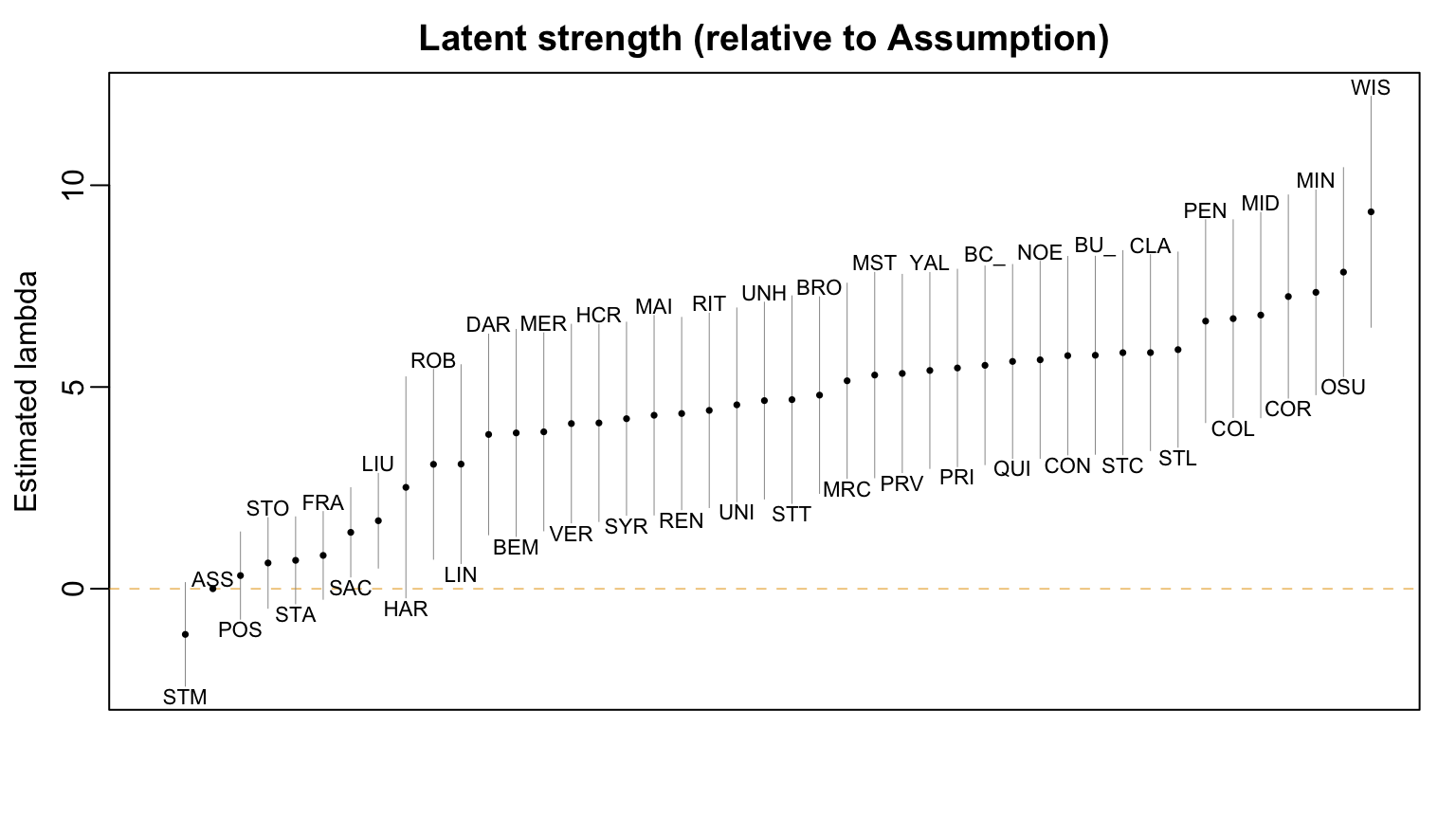
The function BTabilities() returns a matrix with columns containing the estimated value of \(\lambda\) for each team and the associated standard error. Taking a look at the first few rows, we can verify that BTm set Assumption College’s latent strength to be 0. We further see that the model estimates the next several teams as having very large \(\lambda\)’s, suggesting that they are very likely to beat Assumption.
                   ability     s.e.
Assumption        0.000000 0.000000
Bemidji State     3.861526 1.282782
Boston College    5.537068 1.230659
Boston University 5.786624 1.226730
Brown             4.798288 1.217776
Wisconsin, Ohio State, Cornell, and Minnesota all have even larger positive estimated strengths. This is not especially surprising, as these are four of the better teams in the country[^frozenfour].
Figure 1 visualizes the estimated latent strength of each team relative to Assumption. We see the vast majority of the estimates are positive and many of the 95% confidence intervals do not cross 0, indicating that most teams are favored against Assumption.
par(mar =c(3,3,2,1), mgp =c(1.8, 0.5, 0))oi_colors <-palette.colors(palette ="Okabe-Ito")n_teams <-nrow(lambda_hat)y_limit <-range(c(lambda_hat[,1] -2*lambda_hat[,2], lambda_hat[,1] +2*lambda_hat[,2]))ix <-order(lambda_hat[,1])plot(1, type ="n", main ="Latent strength (relative to Assumption)",xlim =c(0, n_teams), ylim = y_limit,xaxt ="n", xlab ="",ylab ="Estimated lambda")abline(h =0, col = oi_colors[2], lwd =0.5, lty =2)for(i in1:n_teams){lines(x =c(i,i), y = lambda_hat[ix[i],"ability"] +c(-2,2) * lambda_hat[ix[i], "s.e."],col = oi_colors[9], lwd =0.5)points(x = i, y = lambda_hat[ix[i],"ability"], pch =16, cex =0.5, col = oi_colors[1]) team_name <-rownames(lambda_hat)[ix[i]] abbr <- team_abbr |> dplyr::filter(team == team_name) |> dplyr::pull(abbr)if(i %%2==0){text(x = i, y =0.25+ lambda_hat[ix[i], "ability"] +2* lambda_hat[ix[i], "s.e."],labels = abbr, cex =0.7) } else{text(x = i, y =-0.25+ lambda_hat[ix[i], "ability"] -2* lambda_hat[ix[i], "s.e."],labels = abbr, cex =0.7) }}
1
Get the number of teams and range of \(\hat{\lambda}\)’s
2
Sort the \(\hat{\lambda}\)’s in increasing order and get the indices
3
Confidence interval for \(\lambda_{j}\) formed by taking the point estimate \(\pm 2\) standard errors
Figure 1: Most teams are favored against the reference team (Assumption College)
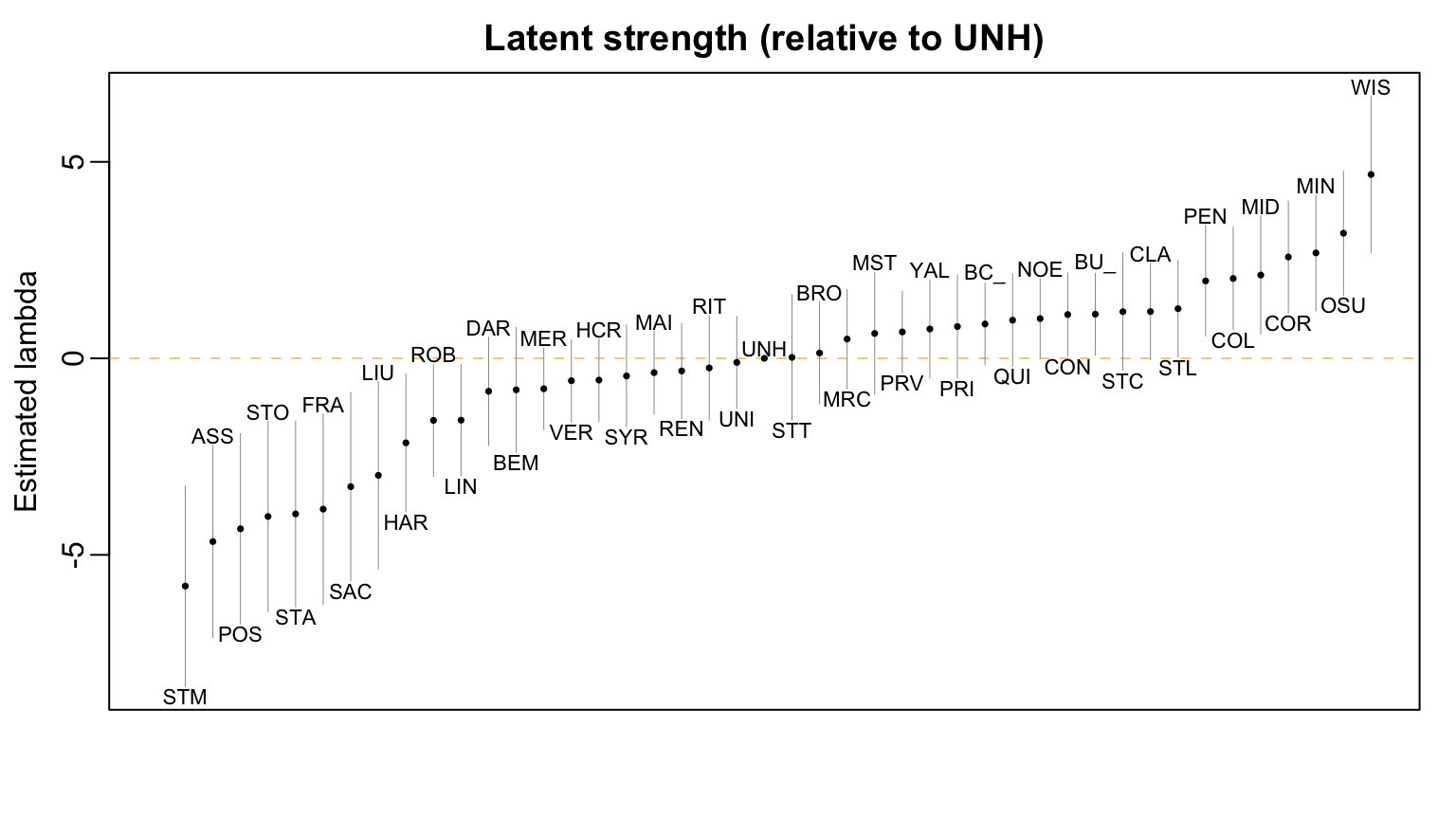
Instead of using Assumption College as the reference, we can re-center our estimated \(\hat{\lambda}_{j}\)’s using the function update()
                ability      s.e.
Assumption    -4.662547 1.2191462
New Hampshire  0.000000 0.0000000
Wisconsin      4.679297 0.9932217
Ohio State     3.184629 0.7887300
Visualizing these shifted \(\hat{\lambda}_{j}\)’ we find that some teams are significantly stronger than New Hampshire and others are substantially weaker.
Figure 2: Some teams are significantly stronger and some teams are significantly weaker than New Hampshire
Simulating a Best-of-5 Series
According to our model estimates, the probability that Wisconsin beats Ohio State in a single game is about 81%
We can use a simulation to estimate the probability that Wisconsin would defeat Ohio State in a best-of-5 series. We first develop code to simulate the series, recording the eventual winner and the number of games needed to be played. For this simulation, we use a while() loop in which each iteration involves simulating a single game. While running this loop, we keep a running tally of each teams’ wins (wi_wins and osu_wins) as well as the number of games played game_counter. We want to iterate through the loop until either (i) wi_wins == 3 & osu_wins < 3 (Wisconsin wins the series) or (ii) osu_wins == 3 & wi_wins < 3 (Ohio State wins the series).
Initialize the number of games played to 0. This counter is incremented in every loop iteration
4
We simulate a game only if the series is not yet decided
5
Simulate outcome of the match: outcome = 1 means Wisconsin won and outcome = 0 means Ohio State won
6
Increment running tallies of each teams’ wins based on outcome
Series ended after 4  games. Winner =  Wisconsin
Wisconsin:  3  Ohio State:  1
Game results: 1 1 0 1 NA
In this single simulation, Wisconsin loses the first game, wins the second and third game, loses the fourh game, and wins the fifth game. To estimate the probability that Wisconsin wins a 5 game series, we can repeat this simulation many, many times. In the following code block, we create a data frame series_results whose rows corresponding to individual simulation replications and which contains two columns, one recording the winner and the other recording the number of games played to determine the winner.
Since \(\mathbb{P}(\textrm{Wisconsin beats Ohio State})\) does not change across simulation iterations, we define this outside the main loop
2
At the beginning of each simulation, we need to re-initialize the running tallies of each team’s wins and the number of games played
3
Since we’re only interested in the ultimate winner and number of games played, there is no need to save the individual match outcomes. But if you want to estimate the probability that Wisconsin wins the series but loses the first game, you’ll need to save individual match outcomes.
Across the 5000 simulated series, Wisconsin won about 95% (4768/5000). We further estimate that the series ends in 3 games with probability 55% (2767/5000), 4 games with probability 32% (1585/5000), and 5 games with probability 13% (648/5000).
table(series_results$Winner)
Ohio State  Wisconsin
       232       4768
table(series_results$Games)
   3    4    5
2767 1585  648
Looking Ahead
Some of the games in our dataset were played at team’s home venue (e.g., La Bahn arean here in Madison) while other games were played a neutral venue (e.g., the championship round of the Beanpot, which is typically played at T.D. Garden in Boston). Our initial Bradley-Terry model does not account for any potential home-ice advantage. In Lecture 13, we will add an term to our model that is 1 if the a game was played at one of the teams’ home and is 0 if it was played a netural site.
We will then simulate a more complex, single-elimination tournament and use the simulation to estimated probabilities of events like “Wisconsin reaches the semi-finals”. To facilitate this, we will save the data table no_ties for future use
In a “best of” series, teams play each other until one has won a majority of the contests. So, in a “best-of-5” series, the first team to reach 3 wins is declared the series winner. For more, check out the Wikipedia entry.↩︎
That is, manually computing 1/(1 + exp(-1 * (lambda[i] - lambda[j]))) for every pair of (i,j).↩︎
Many competitions features a round-robin “group stage” with the top-2 finishers for each group advancing to a single-elimination tournament to decide the champion.↩︎
The Beanpot is a good example: it is a tournament played by teams from schools in the Greater Boston area.↩︎
There are extensions of the Bradley-Terry model that include ties. But the software we’ll be using in this class does not yet support fitting such extensions. So, we will exclude these games from our analysis↩︎