In Lecture 6, we introduced a state-based representation of baseball: each half-inning consists of several at-bats, each of which can be characterized by (i) the number of outs and (ii) configuration of the base-runners. We then estimated the expected number of runs that team can expect to score following at-bats that begin in each of the 24 combinations of outs and base-runner configurations. Today, we will focus less on evaluating what happens in each at-bat (e.g., using run expectancy or run value) and more on how the game transitions from state-to-state.
To motivate our work, let’s reconsider our running example from Lecture 6, the March 20, 2024 game between the Dodgers and Padres. Specifically, let’s load the table atbat2024 created in Lecture 7 and look at the sequence of game states that the Dodgers visited during the 8th inning.
We see that the inning consisted of 8 at-bats. During the first at-bat, in which Max Muncy was walked, the game transitioned from the state 0.000 (i.e., no outs and no runners on base) to the state 0.100 (i.e., no outs and a runner on 1st). During the 6th at-bat, when Mookie Betts drove in a run off a single, the game state did not change: at the beginning and end of the at-bat there was 1 out and runners on 1st and 2nd base.
If we were to replay this half-inning over and over again, how often would the half-inning end after 8 at-bats? How often would the the first at-bat result in a batter reaching first base? And how unusual is it to reach the state 0.111 from the state 0.110?
In this lecture, we will build a Markov chain model, which is a simple probabilistic model of state transitions, to answer such questions. We briefly introduce the relevant mathematical details about Markov chains in Section 2 and work through some simple examples of Markov chains with two (Section 2.1) and three (Section 3.2) states. Then in Section 4, we build a Markov chain model to simulate an entire half-inning of baseball. Using this simulation, we study the distributions of the number of at-bats in a half-inning (Section 4.3) and the number of runs scored in a half-inning (Section 4.4). Finally, in Section 6, we will lean on some mathematical properties of absorbing Markov chains to estimate how many more at-bats a team can expect to face given the current game state.
Data Preparation
The first at-bat in any half-inning of baseball has a deterministic starting state: 0.000, with no outs and no runners on base. The starting state of the next at-bat is, in contrast, non-deterministic. Sometimes the first batter gets out out, in which the game transitions to the state 1.000. But other times, the first batter gets base on with single (0.1000), double (0.010), or triple (0.001). More rarely, the batter scores a home run and the game state remains at 0.000. Put another way, although the first game state visited in a half-inning is deterministic, the second game state visited is random.
From each possible second state, the game could move into multiple possible third states. Continuing this logic until the end of the half-inning, when the game state has Outs = 3 and BaseRunner is undefined, the whole sequence of states visited is stochastic. So, if a team were to play the half-inning over and over again, the exact number of states visited (i.e., at-bats) and the precise sequence might vary from repetition to repetition. Markov chains offer a conceptually simple way to model the randomness of the sequence of game states visited in a half-inning.
To build a Markov chain model for baseball, we need to record the starting and ending state of every at-bat in the 2024 regular season. Recall that in our data table atbat2024, the variable GameState records the value of \(G_{t}\) and was formed by concatenating the variables Outs and BaseRunner. In the code below, we create the variable end_GameState recording the ending state of each at-bat.
For simplicity, we will set end_BaseRunner = "000" when end_Outs == 3 (i.e., the inning is over).
It will later be convenient for us to keep a table listing the single game states as well as the corresponding number of outs and baserunner configurations.
Remove impossible combinations like 3 outs and runners on 1st and 2nd base.
Markov Chains
Let us denote the game state at the start of at-bat \(t\) of a half-inning as \(G_{t}.\) There are 25 possible values for each \(G_{t}\): the 24 different combinations of Outs (0,1, and 2) and BaseRunner (“000”, “100”, “010”, “001”, “110”, “101”, “011”, and “111”) and the one state corresponding to the end of the half-inning. As discussed in Section 1, although \(G_{1}\) is always equal to 0.000, the remaining \(G_{t}\)’s are random and the length of the sequence of states visited in the half-inning is also random.
Formally, this involves coming up with a joint probability distribution for the (possibly infinite) sequence \(G_{1}, G_{2}, \ldots.\) That is, for every possible sequence of states visited, we would need to assign a probability. Once we do this, we could compute things like the probability of a half-inning lasting at least 5 at-bats by finding all sequences of length 5 or more and adding up the corresponding probabilities. Similarly, if we wanted to know the probability that the half-inning began by visiting the states 0.000, 0.100, 0.110, and 0.111, we would find all sequences with that starting sub-sequence and add up the corresponding probabilities.
Of course, calculating the probability for every possible sequence of every possible length is practically impossible. Luckily, it turns out that the probability distribution of a (possibly infinite) sequence of random variables \(\{G_{t}\}\) is fully determined by the sequence of conditional distributions of the form \(G_{t} \vert G_{t-1}, \ldots, G_{1}.\) In other words, it suffices to specify a probability distribution over the next state visited based on its past history.
A Markov chain is a probabilistic model in which the probability of the next state visited depends only on the current state and not all the previous states.
Definition: Markov Chain
A sequence of random variables \(\left\{X_{t}\right\}_{n = 1}^{\infty}\) is called a Markov chain if for all \(t \geq 1\), all sets \(A,\) and trajectories \(x_{1}, \ldots, x_{t-1}\)\[
\mathbb{P}(X_{t} \in A \vert X_{t-1} = x_{t-1}, \ldots, X_{1} = x_{1}) = \mathbb{P}(X_{t} \in A \vert X_{t-1} = x_{t-1}).
\]
When the set of states is discrete (e.g., game states in baseball), Markov chains are fully characterized by a transition probability matrix. If there are \(S\) different states, labelled without loss of generality as \(s = 1, \ldots, S,\) then the \((s,s')\) entry of the transition probability matrix is exactly \(\mathbb{P}(X_{t} = s' \vert X_{t-1} = s)\), the probability of transitioning from state \(s\) to state \(s'.\)
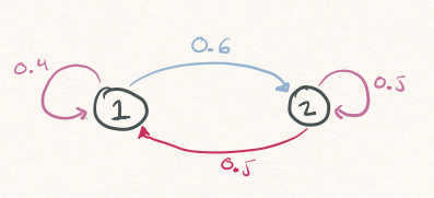
Example: A 2-state Markov Chain
Suppose a system exists in one of two states 1 and `2. Further suppose that
When the system is in state 1, it can remain there with probability 0.6 and it can move to state 2 with probability 0.4.
When the system is in state 2, it remains there with probability 0.5 and it moves to state 1 with probability 0.5.
If we let \(X_{t}\) be the state of the system at time \(t,\) the transition matrix for the Markov chain \(\{X_{t}\}\) is \[
\begin{pmatrix}
0.6 & 0.4 \\
0.5 & 0.5
\end{pmatrix}
\]
The following code simulate 10 time steps from this Markov chain starting from the state 2
Setting byrow = TRUE forces R to build the matrix in row-major order instead of column-major (see this Wikipedia entry)
3
Look up the current state and probabilities of moving to every other state from it. Note that this is a row of the transition matrix.
4
Sample the next state based on the relevant row of the transition matrix
[1] 2 1 1 1 2 2 2 1 1 2
A Graphical Perspective
We can visualize transition probability matrix \(\boldsymbol{\mathbf{P}}\) with a directed graph whose vertices correspond to the distinct states and whose edges are weighted by the corresponding transition probabilities. In the graph, the edge from vertex \(s\) to \(s'\) is the assigned a weight of \(p_{s,s'},\) which is the \((s,s')\) entry of \(\boldsymbol{\mathbf{P}}\) and equals the probability of moving to state \(s'\) from state \(s.\)Figure 1 illustrates the graph corresponding to the simple two-state Markov chain from before.
Figure 1: Graphical representation of the transition probabilities in a two-state Markov chain with one absorbing state
We can interpret a Markov chain with transition matrix \(\boldsymbol{\mathbf{P}}\) as a random walk along this graph. Whenever the walk is at vertex \(s\), it picks one of the outgoing edges from \(s\) to follow at a random. The probability that the walk follows the edge from \(s\) to \(s'\)
Absorbing States
Suppose that \(\{X_{t}\}\) is a Markov chain defined over the states \(\{1, 2, \ldots, S\}\) and let \(\boldsymbol{\mathbf{P}}\) be its transition matrix.
Definition: Absorbing State
A state \(s\) is called an absorbing state if for all \(s' \neq s,\)\(\mathbb{P}(X_{t} = s' \vert X_{t-1} = s) = 0\) and \(\mathbb{P}(X_{t} = s \vert X_{t-1} = s) = 1.\)
That is, an absorbing state is one from which there are no out-going transitions: once the chain reaches an absorbing state, it cannot leave. In our baseball analysis, the state 3.000 corresponding to the end of the half-inning is an absorbing.
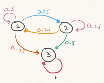
As an illustration, here is the transition matrix for 3-state Markov chain model with one absorbing state (3) \[
\begin{pmatrix}
0.5 & 0.25 & 0.25 \\
0.25 & 0.25 & 0.5 \\
0 & 0 & 1
\end{pmatrix}
\] If the chain is currently in state 1, it (i) remains in state 1 50% of the time and (ii) moves to states 2 25% of the time; and (iii) moves to state 3 25% of the time. If the chain is currently in state 2, it (i) moves to state 1 25% of the time; (ii) remains in state 2 25% of the time; and moves to state 3 50% of the time.
Figure 2 is a graphical illustration of this transition matrix. Notice that the absorbing state 3 only has one outgoing edge that (i) leads back to itself and (ii) has an edge weight of one.
Figure 2: Graphical representation of the transition probabilities in a three-state Markov chain with one absorbing state
The following code simulates 10 steps of the Markov chain beginning in state 1.
In this particular simulation, the chain begins in state 1, moves to state 2, and then moves to the absorbing state 3. The following code block repeats the simulation 10 times, each time starting at state 1 and simulating 10 steps of the Markov chain. Sometimes, the chain immediately moves from 1 to the absorbing state 3. But other times, the chain hops between states 1 and 2 before eventually being absorbed.
Setting seed ensures reproducibility. Allowing the seed to change systematically with replication number ensures we don’t get the exact same results across replications.
2
There is actually no need to introduce the intermediate variables prev_state and next_state
In our 3-state example, let \(T^{A}_{1}\) be the number of steps the chain takes until it hits state 3 starting from state 1: \[
T^{A}_{1} = \min\left\{t \geq 1 : X_{t} = 3\right\}.
\] We can use simulation to study the distribution of \(T^{A}_{1}\) and to estimate quantities like \(\mathbb{P}(T^{A}_{1} > 3)\) or \(\mathbb{P}(T^{A}_{1} = 5).\)
The following code block uses a while() loop to simulate the Markov chain for several iterations until either (i) the absorbing state 3 is reached or (ii) some maximum number of iterations is hit1. Unlike our earlier simulation code, we will not save the full trajectory of states visited. Instead, we will only keep track of the number of iterations needed until the chain reaches state 3.
Maximum number of Markov chain iterations/steps per simulation
3
When running large simulations, it’s helpful to print out your progress after a fixed number of iterations (in this case 100). Sys.time() prints the system time.
4
In each simulation (i.e., iteration of the outer for loop), we need to re-set the counter tracking the number of steps for which we simulate the Markov chain (i.e., iteration counter in the inner while() loop) and re-set the current_state variable to the starting state (in this case, 1).
5
Before starting each iteration, the while() loop checks that the chain isn’t in state 3 and we haven’t yet hit the maximum number of iterations.
6
R evaluates the whole expression on the right-hand side of the <- before assigning it to whatever is on the left-hand side. So, there is no danger here of simultaneously accessing and over-writing the variable current_state, which appears on both sides.
7
In a while() loop, it’s imperative to increment the iterator!
8
The condition fails only when the chain has not reached the absorbing state within the maximum number of allowed iterations (max_iterations).
[1] "Simulation 1000 at 2025-10-20 09:20:02.134454"
[1] "Simulation 2000 at 2025-10-20 09:20:02.146503"
[1] "Simulation 3000 at 2025-10-20 09:20:02.157791"
[1] "Simulation 4000 at 2025-10-20 09:20:02.167222"
[1] "Simulation 5000 at 2025-10-20 09:20:02.176672"
[1] "Simulation 6000 at 2025-10-20 09:20:02.187637"
[1] "Simulation 7000 at 2025-10-20 09:20:02.196892"
[1] "Simulation 8000 at 2025-10-20 09:20:02.207834"
[1] "Simulation 9000 at 2025-10-20 09:20:02.217877"
[1] "Simulation 10000 at 2025-10-20 09:20:02.228788"
Because there are only 3 states and the probabilities of transitioning to state 3 from states 1 and 2 are relatively high, simulating the Markov chain until it hits state 3 takes very little time. Tabulating the different values in absorption_time, we see that the chain
Immediately transitioned from state 1 to state 3 in one step (so that \(T^{A}_{1} = 2\)) in 2440 of the 10,000 simulations
Reached state 3 in exactly two steps (so \(T^{A}_{1} = 2\)) in about 3200 of the 10,000 simulations
Reached state 3 after 20 or more steps in just 2 of the 10,000 simulation
Always reached state 3 within the maximum number of iterations (as indicated by the fact that there are no NA values in absorption_time)
Our goal is to build a Markov chain model for a half-inning of baseball. The fundamental feature of Markov chains is that the state the chain visits next depends only on its current state and not on any of the previously visited states. This is known as the Markov property. Put more somewhat more poetically, the Markov property means that the future depends only on the present and not on the past. In a baseball context, this would mean that what happens after the game reaches any particular state does not depend on what ultimately lead to the current state. So, for instance, when predicting what might happen after the game reaches the state 2.110, with runners on 1st and 2nd base and two outs, it doesn’t matter whether the state was reached from 1.110 or 2.100.
It is important to note, we are assuming that the Markov property holds.
Ultimately, we must estimate the transition probabilities between every pair of the 24 non-absorbing states and the absorbing state corresponding to the end of the half-inning. Because the 9th inning (and any extra innings) can end before a team has amassed three outs2, we exclude all data from the 9th inning and beyond.
A natural estimate of the the probability for transitioning from state \(s\) to the state $s’ $ is divide the number of at-bats that start in state \(s\) and end in state \(s'\) by the number of at-bats that start in state \(s.\)
We first build a table that counts the number of at-bats starting in every state
Next, by grouping by each of GameState and end_GameState, we can count the number of times an at-bat started in some state \(s\) and ended in state \(s'.\)
To compute our transition probability estimates, we start by enumerating all possible combinations of starting and ending state. Then, we will append columns containing the starting state counts n_start and the counts of each pair of state transitions (i.e., n_start_end). For certain pairs of transitions that do not appear in our data (e.g., 0.000 to 3.000), we will manually set n_start_end = 0. Finally, we will divide n_start_end by n_start
Enumerate all 625 possible combinations of starting and ending states of an at-bat
2
Append columns with the number of at-bats (i) starting in each state and (ii) starting & ending in each combination of states
3
Manually set n_start_end = 0 for transitions that are not observed in the data
4
Estimate the transition probability
It is perhaps unsurprising to see that some of the highest transition probabilities are from 2-out states (e.g., 2.000 or 2.100) to the absorbing 3-out state.
To form a transition matrix, we will first “widen” the table transitions using the function tiyr::pivot_wider(). We see that each row of the resulting, temporary table, which we call tmp, corresponds to a starting game state value and there are columns for each of the ending game states.
Looking at these selected entries, we find that the estimated transition probability from 0.000 to 2.000 is zero. This makes some intuitive sense as the batting team cannot, with no outs and no runners on base, lost two outs in a single at-bat. We also see that the transition probabilities from 1 out states (e.g., 1.000 and 1.1000) to the no-out states (e.g., 0.000, 0.110, etc.) are also estimated to be zero. Transitions like 0.100 to 0.000 correspond to situations in which the at-bat begins with a runner on first base and ends with the batter hitting a homerun and driving in the runner.
We can now turn this table into a matrix row and column names are the possible starting and ending game states, we will drop the column GameState from tmp, convert it into a matrix, and then assign the rownames.
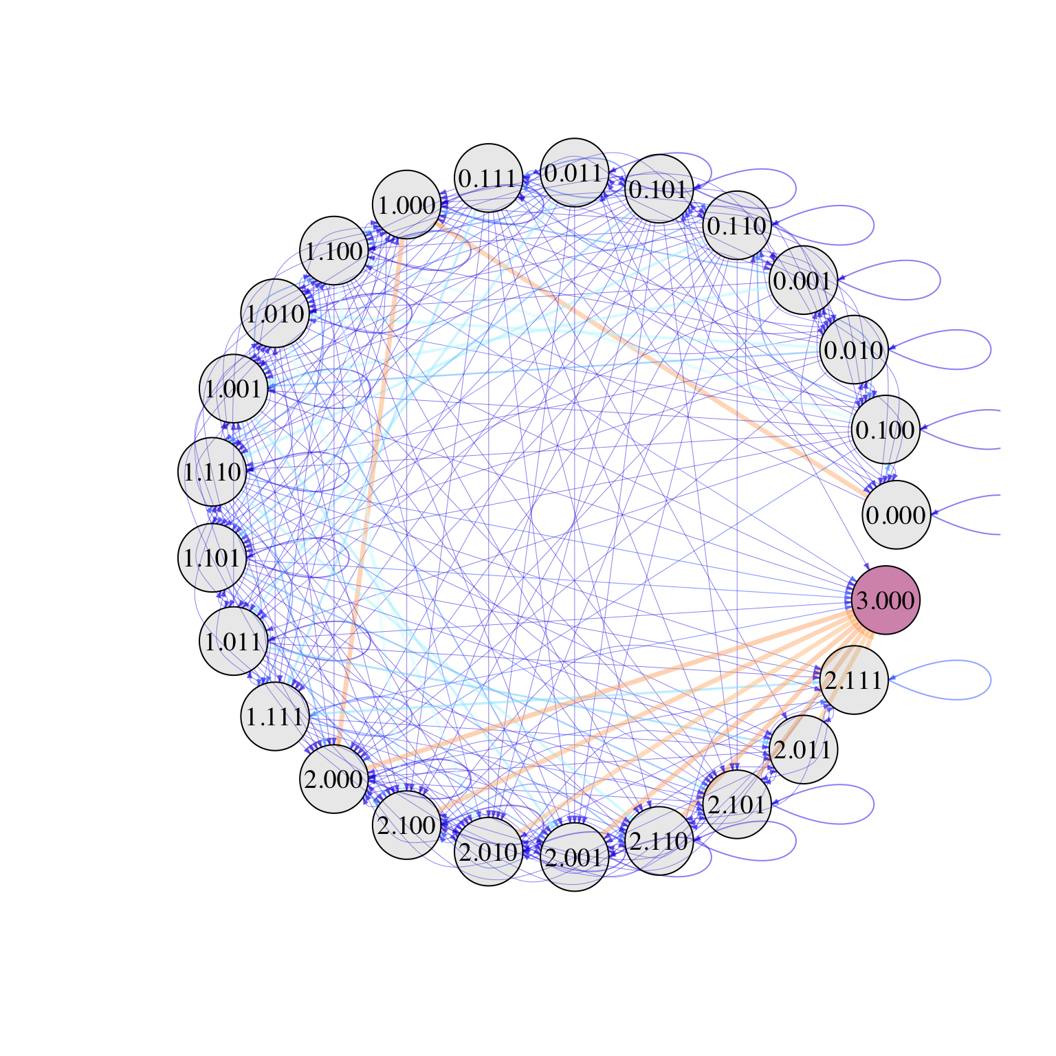
Figure 3 shows a graphical representation of the transition matrix between the game states in baseball. In the figure, the color and thickness of each edge between different states is proportional to corresponding edge transition probabilities, with colors range from blue (0%) to red (100%). So that they are more readily apparent, we have highlighted the self-edges.
Attaching package: 'igraph'
The following objects are masked from 'package:stats':

    decompose, spectrum
The following object is masked from 'package:base':

    union
Figure 3: Graphical representation of transitions between game states in baseball
Simulating a Half-Inning
Now that we have estimated the transition probabilities between all pairs of game states, we are in a position to simulate a single half-inning of baseball. In the following code, we set the initial state to 0.000, since an innings begins with no outs and no runners on base. Then, we use a while() loop to simulate a Markov chain that randomly walks between the states (according to the transition matrix) until it hits the absorbing state 3.000. We set the maximum iterations to be 30, which is an admittedly gross over-estimate on the number of at-bats that can take place in a single half-inning.
This simulated half-inning consisted of 5 at-bats. The first at-bat started in state 0.000 and ended in 0.010, which means that the first batter in the inning hit a double. The second at-bat started in state 0.010 but ended in 1.010, which means that the second batter got out. Similarly, the third at-bat moved the game from 1.010 to 2.010, which means that the third batter also got out. During the fourth simulated at-bat, however, the game state transitions from 2.010 to 2.000. The only way for this to happen is for the batter to score and drive in the runner who was initially on second.
Length of a Half-Inning
Like we did in Section 3.2, we can use simulation to estimate the distribution of the number of at-bats in a half-inning. Unlike that simulation, however, we will keep track of the whole sequence of states visited instead of the absorption time.
Here are the first several rows of states_visited, which record the sequence of game states reached in some of our simulations
states_visited[1:10, 1:8]
      [,1]    [,2]    [,3]    [,4]    [,5]    [,6]    [,7]    [,8]
 [1,] "0.000" "1.000" "2.000" "3.000" NA      NA      NA      NA
 [2,] "0.000" "1.000" "2.000" "2.100" "3.000" NA      NA      NA
 [3,] "0.000" "1.000" "1.100" "2.100" "2.011" "3.000" NA      NA
 [4,] "0.000" "1.000" "2.000" "3.000" NA      NA      NA      NA
 [5,] "0.000" "1.000" "1.100" "3.000" NA      NA      NA      NA
 [6,] "0.000" "1.000" "2.000" "3.000" NA      NA      NA      NA
 [7,] "0.000" "1.000" "2.000" "3.000" NA      NA      NA      NA
 [8,] "0.000" "1.000" "2.000" "2.100" "3.000" NA      NA      NA
 [9,] "0.000" "1.000" "1.100" "2.010" "2.100" "2.110" "3.000" NA
[10,] "0.000" "0.010" "1.001" "1.100" "2.100" "3.000" NA      NA
We find, for instance, that in simulations 1, 4, 6, and 7, the pitching team retired the batting side in 3 at-bats. In Simulation 5, the last at-bat began in the state 1.100 and ended in 3.000. From this we infer that the last at-bat involved an inning-ending double play.
To determine how many at-bats there were in each simulated half-inning, we will first determine which entry in every row is equal to 3.000. In the case of simulation 1, for instance, 3.000 is the 4th entry of row 1. Since the inning ends as soon as the game enters the state 3.000, we need to subtract one from this number to compute the number of at-bats in the half-inning.
In 19,138 of our 50,000 simulations, the inning ended after exactly 3 at-bats. And in 46413 the inning ended with 6 or fewer at-bats. Interestingly, there are two simulations in which the half-inning included 15 at-bats. Here is the sequence of states visited in that first simulation
In this simulated half-inning, the batting team drove in runs in the 4th, 6th, 7th, 8th, 9th, 13th, and 14th at-bats.
Runs Scored in a Half-Inning
To count how runs were scored in each of our 50,000 simulated half-innings, we need to determine how many runs were scored during each simulated at-bat. If we let \(O_{t}\) and \(B_{t}\) be the number of outs and runners at the start of at-bat \(t\) and \(O^{\star}_{t}\) and \(B^{\star}_{t}\) be the numbers of outs and runners at the end of at-bat \(t\), it is not difficult to verify that the number of runs scored during at-bat \(t\) is \[
(O_{t} + B_{t} + 1) - (O_{t}^{\star} + B_{t}^{\star}).
\] As an example, suppose at an at-bat starts in state 1.110 and ends in state 1.000. The only way for such a transition to occur is for the batter to hit a homerun and drive in runs from 1st and 2nd base. That is, three runs are scored during such an at-bat. We verify that \(O_{t} = 1, B_{t} = 2, O_{t}^{\star} = 1\) and \(B_{t}^{\star} = 0.\) So, as expected \((O_{t} + B_{t} + 1) - (O_{t}^{\star} + B_{t}^{\star}) = 3.\)
We can elaborate our Markov chain simulation to count the number of runs scored in each at-bat. To do this, we will need to look up how many outs and baserunners there are based on each game-state. Rather than determining this programmatically, we can manually update the table unik_states.
We now elaborate our Markov chain simulation code to (i) get the number of outs and baserunners at the beginning and end of each simulated at-bat and (ii) add the number of runs scored in the at-bat to a running tally of runs scored in the half-inning.
Warning
This code takes several minutes. The lines looking up the number of outs and base-runners corresponding to each game state introduce some computational redundancies.
The \((s,s')\) entry of \(\boldsymbol{\mathbf{P}}\) is the probability that the chain moves from state \(s\) to state \(s'.\) Based on the 2024 MLB season, we estimated that approximately 23% of at-bats that began in the state 1.000 ended in the state 1.100, so \(p_{\textrm{1.000, 1.100}} \approx 0.23\)
transition_matrix["1.000", "1.100"]
[1] 0.2306792
Now suppose we are at the start of an at-bat with one out and no runners on base (i.e., in state 1.000). How likely is it that in exactly two at-bats, we will have two outs and a runner on 1st base (i.e., be in the state 2.100)?
Before answering this question, we consider a somewhat simpler question: What are all the different intermediate states that the game could visit between 1.000 and 2.100? For instance, the batter facing 1.000 could strike out, moving the game to 2.000, and then the next batter could hit a single, moving the game to 2.100. Alternatively, the batter facing 1.000 could hit a single, moving the game to 1.100, before the next batter strikes out, moving the game to 2.100. A somewhat less likely — but still plausible — way to reach 2.100 from 1.000 in two at-bats is for the first batter to hit a single and for the second batter to hit into a force out at second.
More formally, to compute the probability that the game moves from 1.000 to 2.100 in exactly two steps, we must
Multiply the one-step transition probabilities \(p_{\textrm{1.000},s} \times p_{s, \textrm{2.100}}\) to obtain the probability of transitioning from 1.000 to \(s\) to 2.100for all states \(s\).
Sum these two-step probabilities over all possibly intermediate states \(s.\)
That is, we compute \[
\mathbb{P}(\textrm{game moves from 1.000 to 2.100 in two steps}) = \sum_{s}{p_{\textrm{1.000},s} \times p_{s, \textrm{2.100}}},
\] where the sum is taken over all possible states. Because certain states like 0.000 or 3.000 are unreachable from 1.000, the impossible transitions through those states do not contribute to the sum as the term \(p_{1.000,s}\) will be zero.
Looking carefully at this sum, we recognize the familiar form of matrix multiplication. Specifically, the entry corresponding to (1.000,2.100) in the matrix \(\boldsymbol{\mathbf{P}} \times \boldsymbol{\mathbf{P}}\) is precisely the sum above. We find that there is roughly a 26% probability of reaching 2.100 from 1.000:
For any integer \(n\), let \(\boldsymbol{\mathbf{P}}^{n}\) denote the \(n\)-step transition matrix, which we obtain by multiplying \(\boldsymbol{\mathbf{P}}\) with itself \(n\) times. The \((s,s')\) entry of \(\boldsymbol{\mathbf{P}}^{n}\) is the probability that Markov chain beginning in state \(s\) reaches states \(s'\) in exactly\(n\) steps.
To illustrate, here are several entries of \(\boldsymbol{\mathbf{P}}^{2}\)
Starting from 0.000, there is about a 50% chance that the game reaches the state 2.000 after two at-bats3. Similarly, there is about a 50% chance that the inning ends within two batters of an at-bat beginning in state 1.000. Looking at the three-step transition probabilities, we see that the most three most likely outcomes after the first three batters of a half-inning are (i) the inning ended (38%); (ii) the state 2.100 (23.5%); and (iii) the state 2.010 (7.8%)
Now, we turn to a more nuanced questions: starting from state 1.100, what is the probability that we visit the state 2.010 before the end of the half-inning? And about how many times can we visit the state 2.010 before the half-inning ends? To answer these questions, we need to introduce a bit more theory about Markov chains.
First, recall that in our Markov chain model of a half-inning, the state 3.000 is absorbing: once the chain reaches the state (i.e., the inning ends), it remains there and cannot visit any of the other states.
Definition: Absorbing Markov Chain
A Markov chain is called absorbing if it (i) there is at least one absorbing state and (ii) it is possible to go from any state to an absorbing state in a finite number of steps.
It is not difficult to verify mathematically that our Markov chain for the state transitions between at-bats is absorbing. But it is even easier to verify this empirically: in all of baseball, we’ve never not had a half-inning continue indefinitely. Eventually all half-innings ends, reaching the absorbing state 3.000.
Now, suppose we have an absorbing Markov chain defined over the states \(\{1, 2, \ldots, S\}.\) Without losing any generality, let us suppose that the first \(T\) states are non-absorbing and the last \(A = S - T\) states are absorbing. Then, the transition matrix has the form \[
\boldsymbol{\mathbf{P}} = \begin{pmatrix} Q & R \\ 0 & I_{A} \end{pmatrix},
\] where \(Q\) is a \(T \times T\) matrix capturing one-step transition probabilities between non-absorbing states; \(R\) is a \(T \times A\) matrix capturing one-step transition probabilities between non-absorbing and absorbing states; and \(I_{A}\) is the \(A \times A\) identity matrix, with ones along the diagonal and zeros in all other entries.
In our baseball example, there is only \(A = 1\) absorbing state and \(T = 24\) non-absorbing states. The code below extracts the matrix \(Q\)
For an absorbing Markov chain, the fundamental matrix is given by \[
N = (I_{T} - Q)^{-1}.
\]
For any two transient states \(s\) and \(s',\) the \((s,s')\) entry of \(N,\) which we denote as \(n_{s,s'}\) counts the expected number of times visits state \(s'\) after starting from \(s\) before absorption.
N <-solve(diag(24) - Q)round(N[1:5, 1:5], digits =2)
Looking at several entries of the fundamental matrix of our baseball Markov chain, we notice a few things. First, starting from 0.000, we expect the number of times the chain visits 0.100 about 0.25 times and 0.010 0.06 times, on average. We also observe that the diagonal entries all appear to be larger than 1.
Recall that the diagonal entry \(n_{s,s}\) is the expected number of times that an absorbing chain visits state \(s\) after starting from state \(s.\) So, if the chain starts at \(s,\) it necessarily visits \(s\) at least once. These results suggest, for instance, that starting from the state 1.111 the chain will return to the state 1.111 about 0.19 more times, on average. Similarly, starting from 0.000, the chain expects to return to the starting state 0.000 only 0.05 more times, on average.
Summing the entries along the rows of \(N\), we can compute the expected time until the chain is absorbed starting from each state. So, if we are in an at-bat starting with 1.000, we would expect to face a total of 1.84 additional batters before the end of the half-inning
sum(N["1.000",])
[1] 2.843932
Looking Ahead
Exercises
When simulating the number of runs scored in the half-inning, we initialized our Markov chains from 0.000, which is the state at the start of every half-inning. By initializing at some other state — say 1.000 — we can study the distribution of runs scored after an at-bat beginning in that state. Use a Markov chain simulation to estimate the run expectancy for every state and compare it to the matrix we estimated in Lecture 6.
Footnotes
It is possible to construct Markov chains where some absorbing states are never reached from certain initial states. Without a stopping criterion based on the number of iterations, the while() could continue indefinitely.↩︎
For instance, if the home team begins the bottom of the 9th inning tied and their first batter hits a homerun, then the game ends immediately.↩︎
Reassuringly, we see that there is a a 0% chance of the inning ending after two at-bats!↩︎