STAT 479: Lecture 3
Fitting More Complex XG Models
Recap
- In Lecture 2, fit two XG models
- Model 1 accounted for body part
- Model 2 accounted for body part + technique
- Which model is better?
- Which fits the observed data best?
- Which will predict new data best?
Our Simple XG Models
Qualitative Comparisons
- Consider two shots:
- Right-footed half-volley by Beth Mead against Sweden
- Right-footed backheel by Alessia Russo
# A tibble: 2 × 4
  shot.body_part.name shot.technique.name   XG1   XG2
  <chr>               <chr>               <dbl> <dbl>
1 Right Foot          Half Volley         0.111 0.089
2 Right Foot Backheel 0.111 0.103- Model 2 accounts for more factors
- Intuitively expect it is more accurate
Setup & Notation
- Data: \(n\) shots represented by pairs \((\boldsymbol{\mathbf{x}}_{1}, y_{1}), \ldots, (\boldsymbol{\mathbf{x}}_{n}, y_{n})\)
- Outcomes: \(y_{i} = 1\) if shot \(i\) results in a goal & 0 otherwise
- Feature vector: \(\boldsymbol{\mathbf{x}}_{i}\)
- Assumption: Data is a representative sample from an infinite super-population of shots \[ \textrm{XG}(\boldsymbol{\mathbf{x}}) = \mathbb{E}[Y \vert \boldsymbol{\mathbf{X}} = \boldsymbol{\mathbf{x}}] \]
- \(\hat{p}_{i}\): predicted \(\textrm{XG}\) for shot \(i\) from fitted model
- How close is \(\hat{p}_{i}\) to \(y_{i}\)?
Misclassification Rate (Definition)
- \(\hat{p}_{i} > 0.5:\) model predicts \(y_{i} = 1\) more likely than \(y_{i} = 0\)
- Ideal: \(\hat{p}_{i} > 0.5\) when \(y_{i} = 1\) and \(\hat{p}_{i} < 0.5\) when \(y_{i} = 0\)
- If too many \(\hat{p}_{i}\)’s on wrong-side of 50%, model is badly calibrated.
\[ \textrm{MISS} = n^{-1}\sum_{i = 1}^{n}{\mathbb{I}(y_{i} \neq \mathbb{I}(\hat{p}_{i} \geq 0.5))}, \]
Misclassification Rate (Example)
Model 1 misclassification 0.112
Model 2 misclassificaiton 0.112 - Why do Models 1 & 2 have the same misclassification rate???
# A tibble: 3 × 2
  shot.body_part.name   XG1
  <chr>               <dbl>
1 Right Foot          0.111
2 Left Foot           0.114
3 Head                0.112
# A tibble: 14 × 3
shot.body_part.name shot.technique.name XG2
<chr> <chr> <dbl>
1 Right Foot Volley 0.0637
2 Right Foot Normal 0.121
3 Right Foot Half Volley 0.0892
4 Left Foot Overhead Kick 0
5 Left Foot Normal 0.121
6 Head Normal 0.113
7 Left Foot Half Volley 0.0676
8 Left Foot Volley 0.163
9 Head Diving Header 0
10 Right Foot Lob 0.208
11 Right Foot Backheel 0.103
12 Right Foot Overhead Kick 0.0714
13 Left Foot Lob 0
14 Left Foot Backheel 0 Brier Score (Definition)
- MISS only cares whether \(\hat{p}_{i}\) is on the wrong-side of 50%
- Forecasting \(\hat{p} = 0.501\) and \(\hat{p} = 0.999\) have same loss when \(y = 0\)
- Doesn’t penalize how far \(\hat{p}\) is from \(Y\)
- Brier Score penalizes distance b/w forecast \(\hat{p}\) & \(Y\) \[ \text{Brier} = n^{-1}\sum_{i = 1}^{n}{(y_{i} - \hat{p}_{i})^2}. \]
- Just Mean Square Error applied to binary outcomes
Brier Score (Example)
Model 1 Brier Score: 0.1 Model 2 Brier Score: 0.099 Log-Loss (Definition)
- Like Brier but penalizes extreme mistakes more severely
\[ \textrm{LogLoss} = -1 \times \sum_{i = 1}^{n}{\left[ y_{i} \times \log(\hat{p}_{i}) + (1 - y_{i})\times\log(1-\hat{p}_{i})\right]}. \]
- Theoretically, can be infinite (when \(\hat{p} = 1-y\))
- In practice, truncate \(\hat{p}\) to \([\epsilon,1-\epsilon]\) to avoid \(\log(0)\)
- Also known as cross-entropy loss in ML literature
Log-Loss Score (Example)
Model 1 Log-Loss: 0.351
Model 2 Log-Loss: 0.348
Estimating Out-of-Sample Error
In-sample Error
- Recall our setup:
- Data is a sample from super-population \(\mathcal{P}\)
- Fit model to estimate \(\mathbb{E}[Y \vert \boldsymbol{\mathbf{X}} = \boldsymbol{\mathbf{x}}]\)
- Fitted model returns predictions \(\hat{p}(\boldsymbol{\mathbf{x}})\)
- Computed \(\textrm{MISS}, \textrm{Brier},\) and \(\textrm{LogLoss}\) w/ same data used to fit model
- This only checks whether model fits observed data well
- How well does model predict new, previously unseen data?
Out-of-Sample Error
- Say we had a second dataset \((\boldsymbol{\mathbf{x}}_{1}^{\star}, y_{1}^{\star}), \ldots, (\boldsymbol{\mathbf{x}}_{m}^{\star}, y_{M}^{\star})\) from \(\mathcal{P}\)
- Compute predictions \(\hat{p}^{\star}_{m}:= \hat{p}(\boldsymbol{\mathbf{x}}_{m}^{\star})\)
- Important: \((\boldsymbol{\mathbf{x}}_{m}^{\star}, y_{m}^{\star})\)’s not used to fit the model
- Assess how close \(\hat{p}^{\star}_{m}\)’s are to \(y^{\star}_{m}\)’s
- Could use misclassification rate, Brier score, or log-loss
- Result is the out-of-sample loss
Cross-Validation
- Problem: we don’t have access to a second dataset
- Solution: create random training/testing split
- Train on a random subset containing 75% of the data
- Evaluate using the remaining held-out portion
The Training/Testing Paradigm
model1 <-
  train_data |>
  dplyr::group_by(shot.body_part.name) |>
  dplyr::summarise(XG1 = mean(Y))
model2 <-
  train_data |>
  dplyr::group_by(shot.body_part.name, shot.technique.name) |>
  dplyr::summarise(XG2 = mean(Y), .groups = "drop")
train_preds <-
  train_data |>
  dplyr::inner_join(y = model1, by = c("shot.body_part.name")) |>
  dplyr::inner_join(y = model2, by = c("shot.body_part.name", "shot.technique.name"))
test_preds <-
test_data |>
dplyr::inner_join(y = model1, by = c("shot.body_part.name")) |>
dplyr::inner_join(y = model2, by = c("shot.body_part.name", "shot.technique.name"))
logloss(train_preds$Y, train_preds$XG1)
logloss(test_preds$Y, test_preds$XG1)
logloss(train_preds$Y, train_preds$XG2)
logloss(test_preds$Y, test_preds$XG2)BodyPart train log-loss: 0.357 test log-loss: 0.334 BodyPart+Technique train log-loss: 0.355 test log-loss: 0.351 Multiple Splits
- Recommend averaging over many train/test splits (e.g., 100)
- See lecture notes for full code
- Each iteration in a
for()loop:- Sets new seed & form new train/test split
- Re-trains both XG models and computes train & test error
- Save errors in an array
Model 1 training logloss: 0.351
Model 2 training logloss: 0.348
Model 1 test logloss: 0.352
Model 2 test logloss: 0.356 - Simpler model appaers to have slightly smaller out-of-sample log-loss!
Logistic Regression
Motivation: Accounting for Distance
- Model 1 gives same prediction for
- A header from 1m away
- A header from 15m away
- How to account for continuous feature like
DistToGoal?
- Idea: Divide into discrete bins and then average within bins
- Problem: sensitivity to bin sizes (1m , 3m, 10m)
- Problem: potential small sample issues
Logistic Regression
Binary outcome \(Y\) and numerical predictors \(X_{1}, \ldots, X_{p}\): \[ \log\left(\frac{\mathbb{P}(Y= 1 \vert \boldsymbol{\mathbf{X}})}{\mathbb{P}(Y = 0 \vert \boldsymbol{\mathbf{X}})}\right) = \beta_{0} + \beta_{1}X_{1} + \cdots + \beta_{p}X_{p}. \]
Keeping all other predictors constant, a one unit change in \(X_{j}\) associated with a \(\beta_{j}\) change in the log-odds
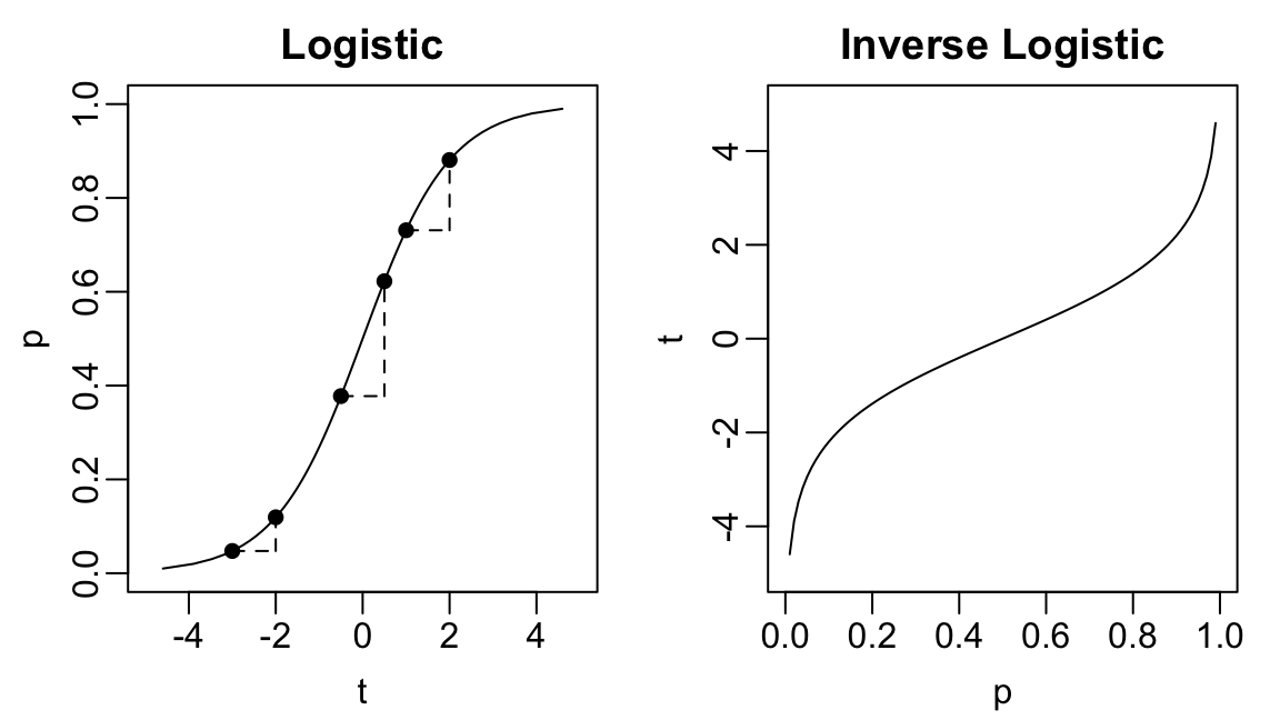
Say \(\beta_{j} = 1\). Increasing \(X_{j}\) by 1 unit moves \(\mathbb{P}(Y = 1)\)
- From 4.7% to 11.2% (log-odds from -3 to -2)
- From 37.8% to 62.2% (log-odds from -0.5 to 0.5)
- From 73.1% to 88.1% (log-odds from 1 to 2)
Logistic & Inverse Logistic Functions
- Logistic function: \(f(t) = [1 + e^{-t}]^{-1}\)
- Inverse logistic: \(f^{-1}(p) = \log{p/(1-p)}\)
An Initial Model
- \(X_{1}\): distance from shot to goal (
DistToGoal) - \(\log\left(\frac{\mathbb{P}(Y = 1)}{\mathbb{P}(Y = 0)} \right) = \beta_{0} + \beta_{1} X_{1}\)
Call:
glm(formula = Y ~ DistToGoal, family = binomial("logit"), data = train_data)

Coefficients:
             Estimate Std. Error z value Pr(>|z|)
(Intercept) -0.134174   0.128410  -1.045    0.296
DistToGoal  -0.127023   0.009115 -13.935   <2e-16 ***
---
Signif. codes:  0 '***' 0.001 '**' 0.01 '*' 0.05 '.' 0.1 ' ' 1

(Dispersion parameter for binomial family taken to be 1)

    Null deviance: 2549.7  on 3569  degrees of freedom
Residual deviance: 2290.7  on 3568  degrees of freedom
AIC: 2294.7

Number of Fisher Scoring iterations: 6
Assessing Model Performance
- Use
predict()to make test set predictions
Dist training logloss: 0.321 Dist testing logloss: 0.305 - Averaging across 100 train/test splits: distance-based model better than body-part-based model
Dist*BodyPart training logloss: 0.3167 Dist*BodyPart testing logloss: 0.3173 Including Multiple Predictors
- Distance-based model is more accurate than body-part based model
- What if we account for body part and distance?
Model Specification
\[ \beta_{0} + \beta_{1}\times \textrm{DistToGoal} + \\ \beta_{\textrm{LeftFoot}}\times \mathbb{I}(\textrm{LeftFoot}) + \beta_{\textrm{RightFoot}} \times \mathbb{I}(\textrm{RightFoot}) \]
Different predictions based on the body part used to attempt the shot
For a shot taken at distance \(d\):
- Header: log-odds: \(\beta_{0} + \beta_{1}d\)
- Left-footed shot: \(\beta_{0} + \beta_{1}d + \beta_{\textrm{LeftFoot}}\)
- Right-footed shot: \(\beta_{0} + \beta_{1}d + \beta_{\textrm{RightFoot}}\)
Fitted Model
fit <- glm(formula = Y~DistToGoal + shot.body_part.name,
           data = train_data, family = binomial("logit"))
summary(fit)
Call:
glm(formula = Y ~ DistToGoal + shot.body_part.name, family = binomial("logit"),
    data = train_data)

Coefficients:
                              Estimate Std. Error z value Pr(>|z|)
(Intercept)                   -0.49847    0.15504  -3.215   0.0013 **
DistToGoal                    -0.17501    0.01081 -16.187  < 2e-16 ***
shot.body_part.nameLeft Foot   1.28091    0.17286   7.410 1.26e-13 ***
shot.body_part.nameRight Foot  1.30351    0.15711   8.297  < 2e-16 ***
---
Signif. codes:  0 '***' 0.001 '**' 0.01 '*' 0.05 '.' 0.1 ' ' 1

(Dispersion parameter for binomial family taken to be 1)

    Null deviance: 2533.3  on 3569  degrees of freedom
Residual deviance: 2167.4  on 3566  degrees of freedom
AIC: 2175.4

Number of Fisher Scoring iterations: 6
Interactions
- Model assumes effect of distance is the same regardless of body part
- Interactions allow the effect of one factor to vary based on the value of another. \[ \begin{align} &\beta_{0} + \beta_{\textrm{LeftFoot}} \times \mathbb{I}(\textrm{LeftFoot}) + \beta_{\textrm{RightFoot}} * \mathbb{I}(\textrm{RightFoot}) + \\ &+[\beta_{\textrm{Dist}} + \beta_{\textrm{Dist:LeftFoot}}*\mathbb{I}(\textrm{LeftFoot}) + \beta_{\textrm{Dist:RightFoot}}\mathbb{I}(\textrm{RightFoot})] \times \textrm{Dist} \end{align} \]
Fitting Interactive Model
fit <-
  glm(formula = Y~DistToGoal * shot.body_part.name,
      data = train_data, family = binomial("logit"))
summary(fit)
Call:
glm(formula = Y ~ DistToGoal * shot.body_part.name, family = binomial("logit"),
    data = train_data)

Coefficients:
                                         Estimate Std. Error z value Pr(>|z|)
(Intercept)                               1.04701    0.41889   2.499  0.01244
DistToGoal                               -0.34422    0.05092  -6.761 1.37e-11
shot.body_part.nameLeft Foot             -0.21195    0.50881  -0.417  0.67700
shot.body_part.nameRight Foot            -0.82193    0.46059  -1.785  0.07434
DistToGoal:shot.body_part.nameLeft Foot   0.16418    0.05457   3.009  0.00263
DistToGoal:shot.body_part.nameRight Foot  0.20871    0.05233   3.988 6.66e-05

(Intercept)                              *
DistToGoal                               ***
shot.body_part.nameLeft Foot
shot.body_part.nameRight Foot            .
DistToGoal:shot.body_part.nameLeft Foot  **
DistToGoal:shot.body_part.nameRight Foot ***
---
Signif. codes:  0 '***' 0.001 '**' 0.01 '*' 0.05 '.' 0.1 ' ' 1

(Dispersion parameter for binomial family taken to be 1)

    Null deviance: 2549.7  on 3569  degrees of freedom
Residual deviance: 2214.5  on 3564  degrees of freedom
AIC: 2226.5

Number of Fisher Scoring iterations: 6
Cross-Validation
- Fit & assess models w/ 100 train/test splits
- Model w/ interactions is slightly better than others
BodyPart training logloss: 0.351
BodyPart+Technique training logloss: 0.348
BodyPart test logloss: 0.352
BodyPart+Technique test logloss: 0.356
Dist*BodyPart training logloss: 0.3167 Dist*BodyPart testing logloss: 0.3173 Dist*BodyPart training logloss: 0.3069 Dist*BodyPart testing logloss: 0.308 Dist*BodyPart training logloss: 0.3047 Dist*BodyPart testing logloss: 0.3066 Random Forests
Including Even More Features
- StatsBomb records many potentially important features
 [1] "shot.type.name"      "shot.technique.name" "shot.body_part.name"
 [4] "DistToGoal"          "DistToKeeper"        "AngleToGoal"
 [7] "AngleToKeeper"       "AngleDeviation"      "avevelocity"
[10] "density"             "density.incone"      "distance.ToD1"
[13] "distance.ToD2"       "AttackersBehindBall" "DefendersBehindBall"
[16] "DefendersInCone" "InCone.GK" "DefArea" - How much more predictive accuracy can we gain by accounting for these?
- Challenge: hard to specify nonlinearities & interactions correctly in
glm()
Regression Trees I
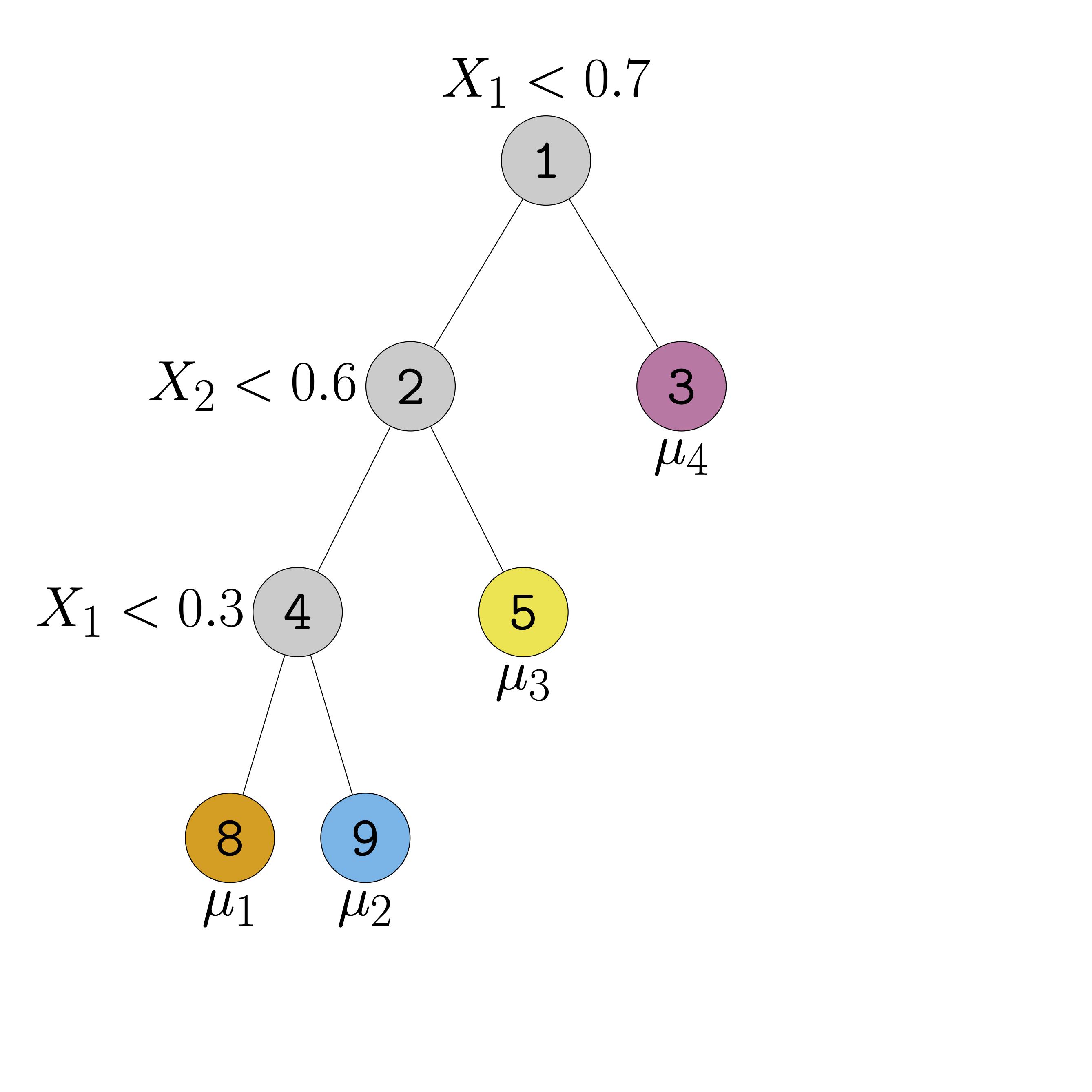
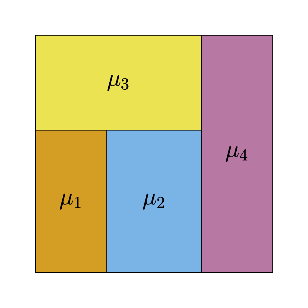
- Regression trees can elegantly model interactions and non-linearities
- Regression trees are just step-functions
Regression Trees II
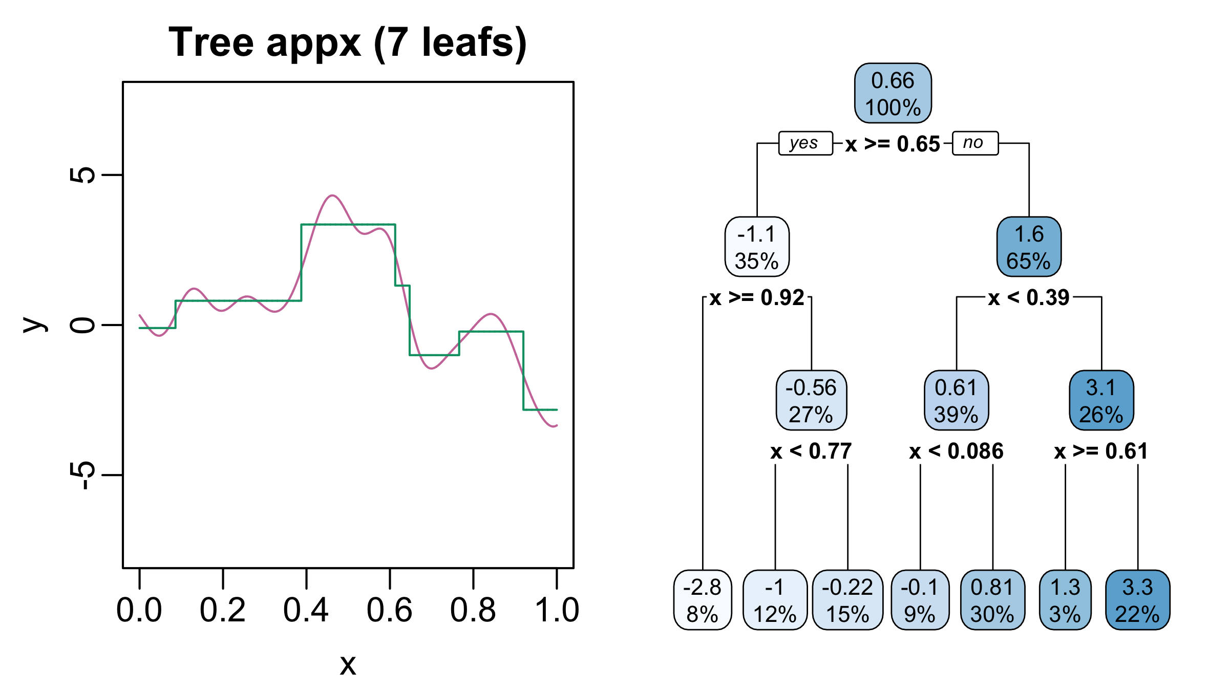
Regression Trees III
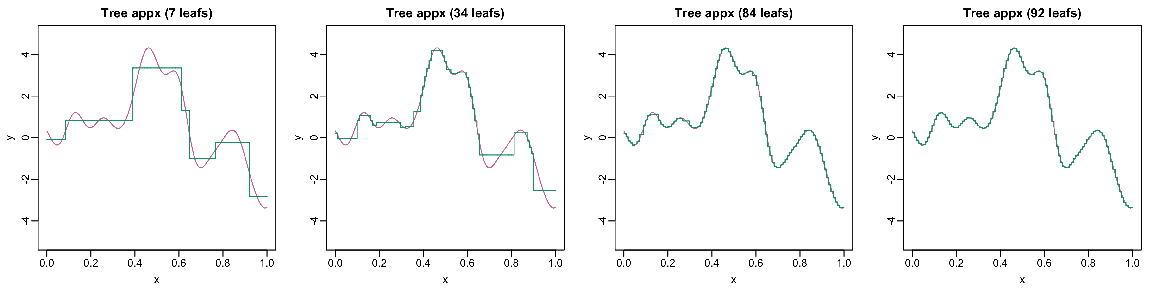
- Regression trees can approximate functions arbitrarily well
- But often need very deep and complicated trees
Tree Ensembles
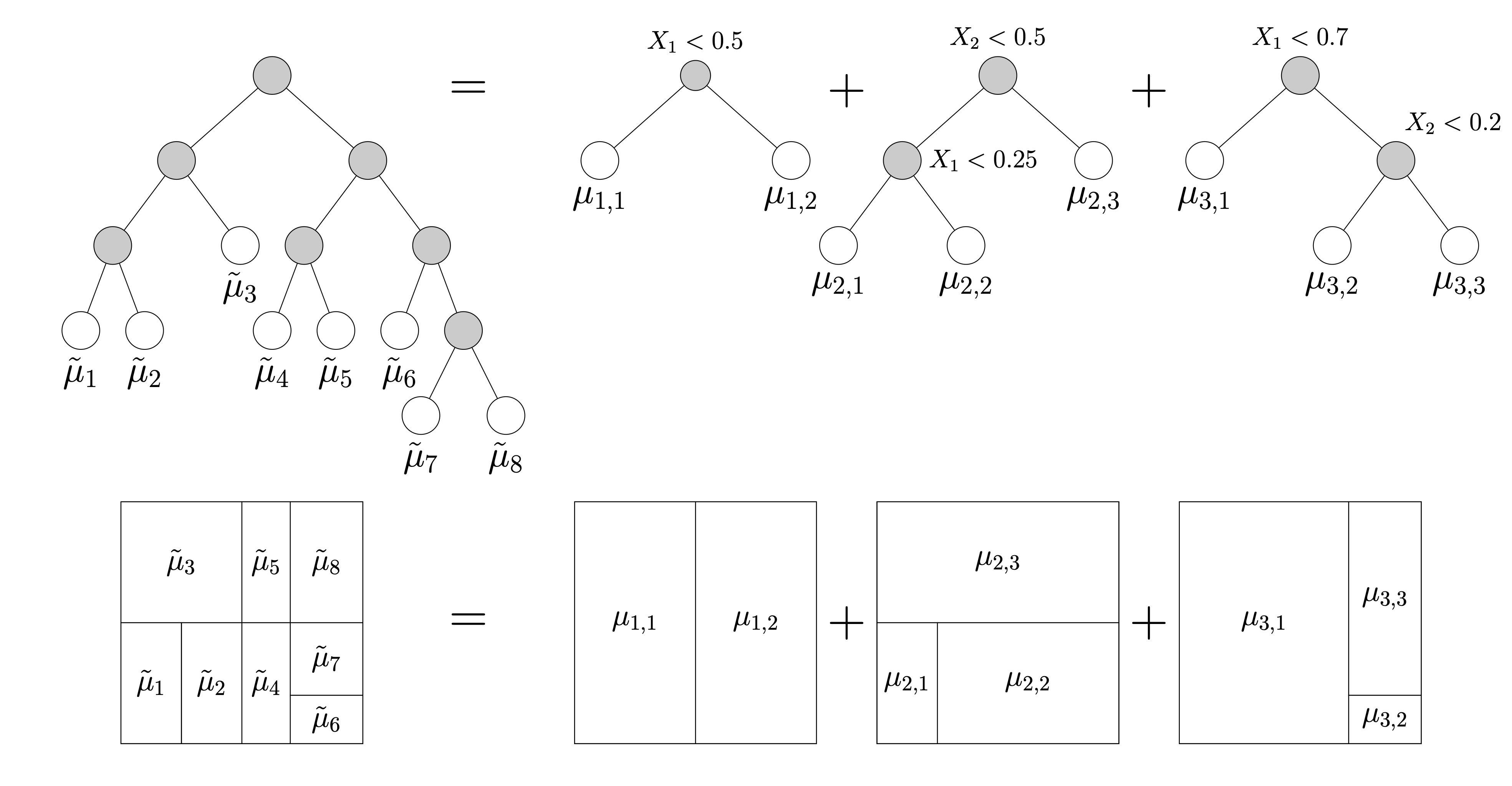
- Complicated trees can be written as sums of shallow trees!
Random Forests
- Approximate \(\mathbb{E}[Y \vert \boldsymbol{\mathbf{X}} = \boldsymbol{\mathbf{x}}]\) w/ tree ensemble
- No need to pre-specify functional form or interactions
- Scales nicely even if \(\boldsymbol{\mathbf{X}}\) is high-dimensional
- We will use implementation in ranger package
Fitting a Random Forests Model
shot_vars <-
  c("Y",
    "shot.type.name",
    "shot.technique.name", "shot.body_part.name",
    "DistToGoal", "DistToKeeper", # dist. to keeper is distance from GK to goal
    "AngleToGoal", "AngleToKeeper",
    "AngleDeviation",
    "avevelocity","density", "density.incone",
    "distance.ToD1", "distance.ToD2",
    "AttackersBehindBall", "DefendersBehindBall",
    "DefendersInCone", "InCone.GK", "DefArea")

wi_shots <-
  wi_shots |>
  dplyr::mutate(
    shot.type.name = factor(shot.type.name),
    shot.body_part.name = factor(shot.body_part.name),
    shot.technique.name = factor(shot.technique.name))

set.seed(479)
train_data <-
  wi_shots |>
  dplyr::slice_sample(n = n_train) |>
  dplyr::select(dplyr::all_of(c("id",shot_vars)))

test_data <-
  wi_shots |>
  dplyr::anti_join(y = train_data, by = "id") |>
  dplyr::select(dplyr::all_of(c("id", shot_vars)))

y_train <- train_data$Y
y_test <- test_data$Y

train_data <-
  train_data |>
  dplyr::mutate(Y = factor(Y, levels = c(0,1))) |>
  dplyr::select(-id)
test_data <-
  test_data |>
  dplyr::mutate(Y = factor(Y, levels = c(0,1))) |>
dplyr::select(-id)Average Out-of-Sample Performance
- Across 100 random train/test splits random forests model outperforms others
RandomForest training logloss: 0.1113 RandomForest testing logloss: 0.2705 Comparison to StatsBomb’s Model
RandomForest training logloss: 0.154 StatsBomb training logloss: 0.2642 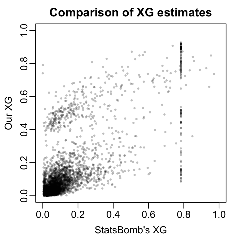
Looking Ahead
- Next week: model-based assessment of NBA player performance
- Good idea to read notes & install hoopR
- Review notes on linear regression from prev. course (e.g., STAT 333 or 340)
- Chapter 1.6 of Beyond Multiple Linear Regression is a great resource as well
- Form projects groups by tomorrow
- Should be able to sign up on Canvas
- Email me if you’re running into issues
- Piazza can help find teammates
- I’ll post several project ideas over the weekend
- Goal for y’all: form ideas of what y’all want to do by end of next week
- Goal for me: check-in w/ all project teams by 9/26