load("statcast2024.RData")
load("runValue2024.RData")
load("player2024_lookup.RData")
oi_colors <-
palette.colors(palette = "Okabe-Ito")Lecture 8: Defensive Credit Allocation in Baseball
Overview
In Lecture 7, we distributed the run value created in each at-bat between the batter and base runners. Aggregating over all at-bats, we computed each player’s \(\textrm{RAA}^{\textrm{br}},\) which quantifies how much more run value a player created through his base running than would otherwise be expected based on the starting game states and ending events of the at-bats in which he was involved. We also computed \(\textrm{RAA}^{\textrm{b}},\) which quantifies how much more run value a player created through his hitting than would be expected based on his position.
According to the conservation of runs framework introduced by Baumer, Jensen, and Matthews (2015), whenever the batting team creates \(\delta\) units of run value in at-bat, the fielding team (necessarily) gives up \(\delta\) units of run value. Equivalently, the fielding team creates \(-\delta\) units of run value. In this lecture, we discuss how to divide this \(-\delta\) run value between the pitchers (Section 6) and fielders (Section 5).
For at-bats \(i\) that end without the ball being put in play (i.e., a strikeout, walk, or a homerun), we will assign the entirety of the \(-\delta_{i}\) run value to the pitcher. But for at-bats that result with balls put in play, we will divide \(-\delta_{i}\) into two parts \(\delta^{(f)}_{i} = -\delta \times \hat{p}_{i}\) and \(\delta^{(p)} = -\delta_{i} \times (1 - \hat{p}_{i})\) where \(\hat{p}_{i}\) is an estimate of the probability that play results in an out given the batted ball’s location (Section 3). We will specifically estimate these out probabilities using Generalized Additive Models (Section 4). Finally, we compute how more run value each player creates through their batting, baserunning, pitching, and fielding than a replacement level player (Section 7).
Hit Location Data
We begin by loading several of the data tables created in Lecture 6 and Lecture 7 including statcast2024, which contains pitch-level data for all regular season pitches in 2024, runValue2024, which contains the \(\delta_{i}\)’s for each regular season at-bat, and player2024_lookup, which contains the names and MLB Advanced Media identifiers for each player.
Recall from Lecture 6 that the Statcast variables hc_x and hc_y record the coordinates where each batted ball is first fielded. When we plotted the available hc_x and hc_y values, we saw the outlines of the park, with home plate located around hc_x = 125 and hc_y = 200. We can also roughly make out the first and third base lines and the infield.
par(mar = c(3,3,2,1), mgp = c(1.8, 0.5, 0))
plot(statcast2024$hc_x, statcast2024$hc_y,
     xlab = "hc_x", ylab = "hc_y",
     pch = 16, cex = 0.2,
     col = adjustcolor(oi_colors[1], alpha.f = 0.1))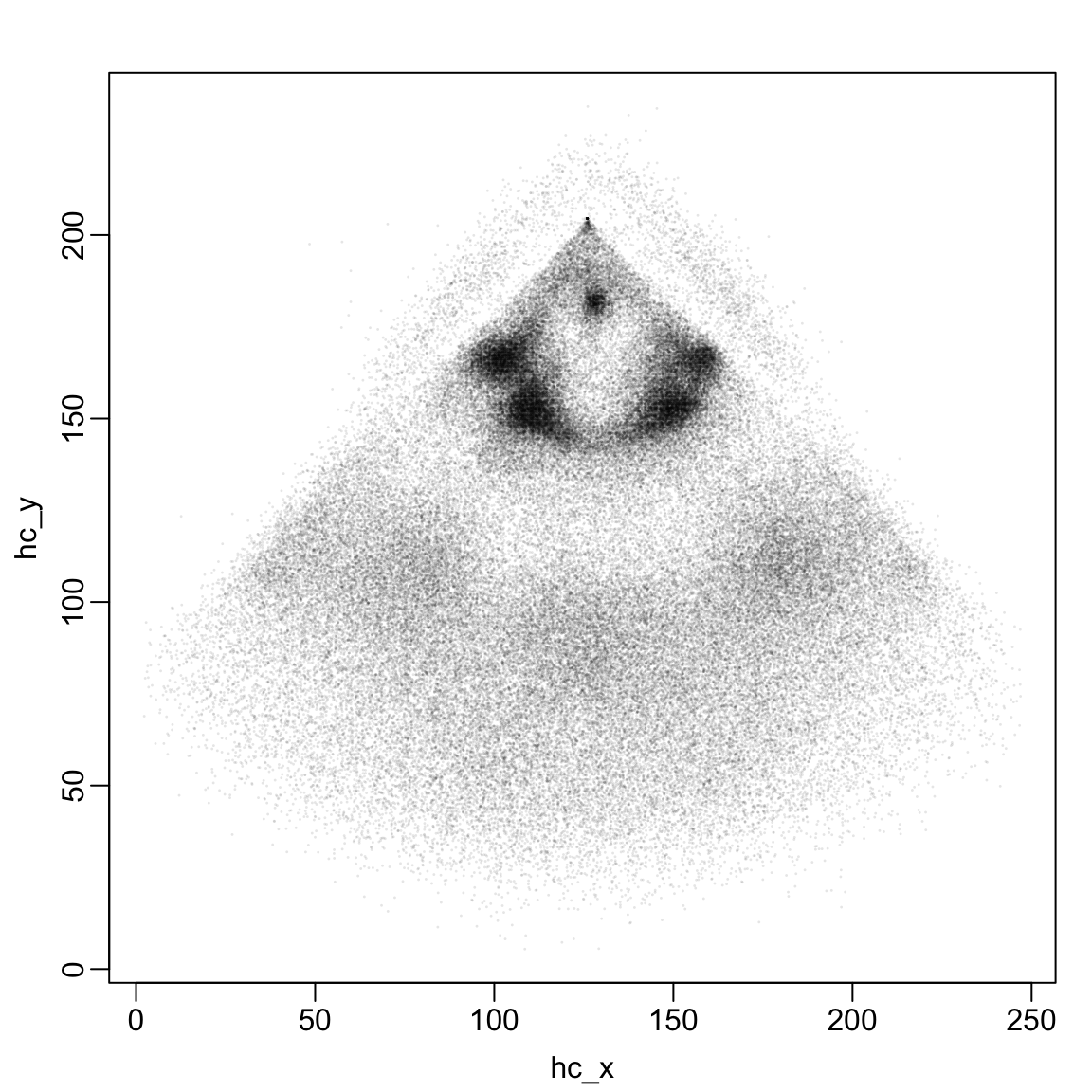
It is not immediately apparent, however, whether the first base line is on the left or right. Luckily, StatCast also contains the official fielding position of the player who first fields the ball1. When we plot just the pitches first fielded by first basemen (hit_location=3), we see that in the original (hc_x, hc_y) coordinate system, first base is on the right hand side of the plot.
par(mar = c(3,3,2,1), mgp = c(1.8, 0.5, 0))
plot(statcast2024$hc_x[statcast2024$hit_location!=3],
     statcast2024$hc_y[statcast2024$hit_location != 3],
     xlab = "hc_x", ylab = "hc_y",
     pch = 16, cex = 0.2,
     col = adjustcolor(oi_colors[1], alpha.f = 0.1))
points(statcast2024$hc_x[statcast2024$hit_location==3],
     statcast2024$hc_y[statcast2024$hit_location==3],
     pch = 16, cex = 0.2,
     col = adjustcolor(oi_colors[2], alpha.f = 0.1))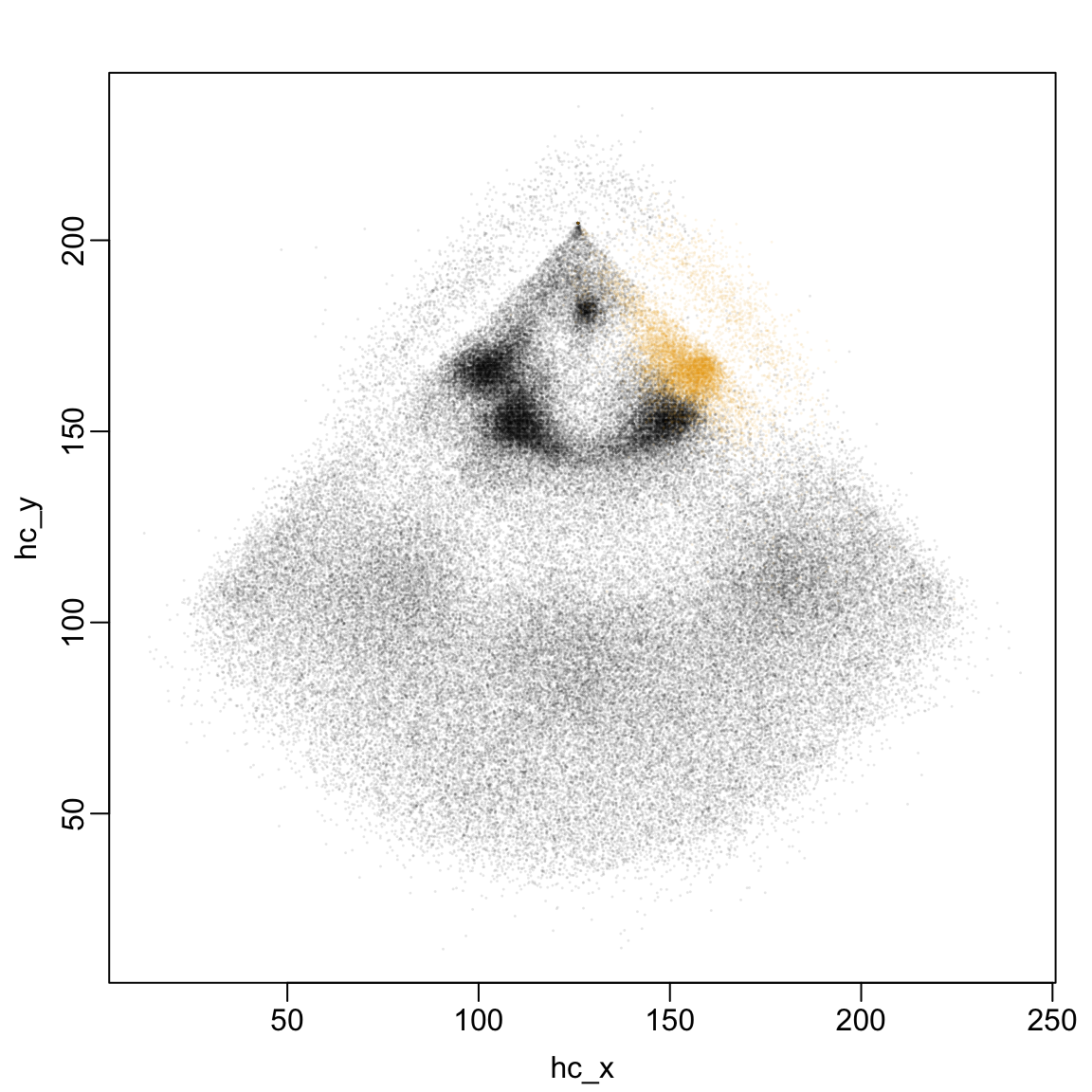
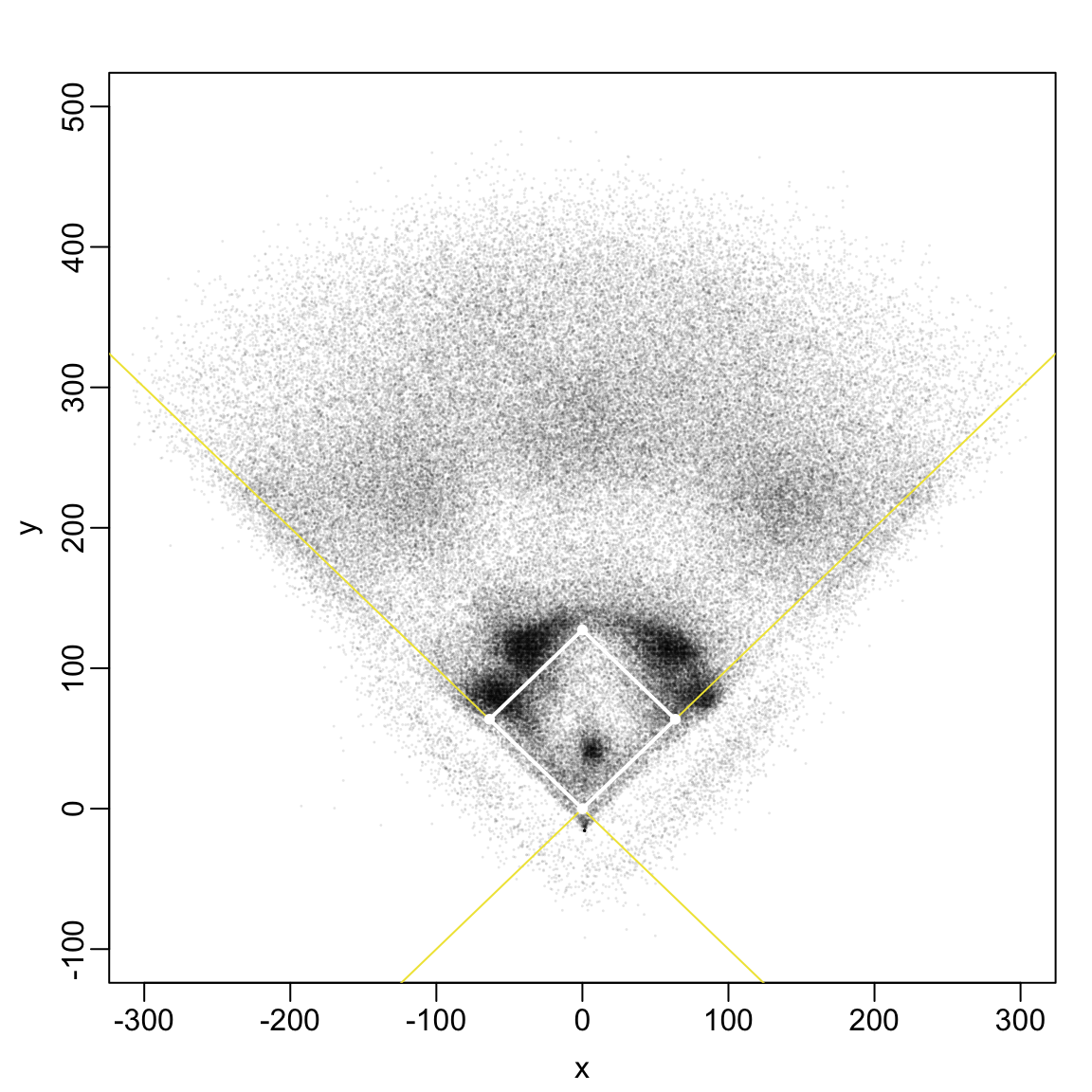
Although MLB Stadiums are equipped with lots of very cool camera and ball tracking technology, the variables hc_x and hc_y are not derived from those technologies. Instead a stringer manually marks the location of the batted ball on a tablet so the coordinates hc_x and hc_y are expressed in units of pixels on that tablet. Jim Albert, who is one of the founding fathers of Statistical research in baseball, suggested the following transformation from the original (hc_x, hc_y) coordinate system to one that places home plate at the bottom of the plot (with coordinates (0,0)) and measures distances in feet. \[
\begin{align}
x &= 2.5 \times (\texttt{hc\_x} - 125.42) & y &= 2.5 \times (198.27 - \texttt{hc\_y})
\end{align}
\]
The following code implements this transformation, storing the new coordinates as x and y and then plots the batted ball locations. It also overlays the first and third base lines, the base paths and places points at the base locations.
statcast2024 <-
statcast2024 |>
dplyr::mutate(
x = 2.5 * (hc_x - 125.42),
y = 2.5 * (198.27 - hc_y))
par(mar = c(3,3,2,1), mgp = c(1.8, 0.5, 0))
plot(statcast2024$x,
statcast2024$y,
xlab = "x", ylab = "y",
pch = 16, cex = 0.2,
xlim = c(-300, 300),
ylim = c(-100, 500),
col = adjustcolor(oi_colors[1], alpha.f = 0.1))
abline(a = 0, b = 1, col = oi_colors[5], lwd = 1)
abline(a = 0, b = -1, col = oi_colors[5], lwd = 1)
lines(x = c(0,90/sqrt(2)), y = c(0, 90/sqrt(2)), col = "white", lwd = 2)
lines(x = c(0,-90/sqrt(2)), y = c(0, 90/sqrt(2)), col = "white", lwd = 2)
lines(x = c(90/sqrt(2), 0), y = c(90/sqrt(2), 90*sqrt(2)), col = "white", lwd = 2)
lines(x = c(-90/sqrt(2), 0), y = c(90/sqrt(2), 90*sqrt(2)), col = "white", lwd = 2)
points(x = 0, y = 0, pch = 16, cex = 0.8, col = "white")
points(x = 90/sqrt(2), y = 90/sqrt(2), pch = 16, cex = 0.8, col = "white")
points(x = -90/sqrt(2), y = 90/sqrt(2), pch = 16,cex = 0.8, col = "white")
points(x = 0, y = 90*sqrt(2), pch = 16, cex = 0.8, col = "white")- 1
-
The function
abline(a,b)plots the line \(y = ax + b\). In our new coordinate system the first and third base lines correspond to the lines \(y = x\) and \(y = -x\). - 2
-
In our new coordinate system, home plate is at
(0,0). First base and third base are 90 feet away from home plate along the 45 degree lines, meaning that their coordinates are(90/sqrt(2), 90/sqrt(2))and (-90/sqrt(2), 90/sqrt(2))`.
In Lecture 7, we created a table atbat2024 that contained the beginning and ending states of each at-bat, run value, ending event, and identities of the batter and baserunners. Today, we will build a similar data frame that contains the ending event, identities of the pitcher and fielders, and, if the at-bat resulted in a ball being put into play, the batted ball locations. Like the code we used to build atbat2024, we need to identify the last entry in the column events in each at bat as well as the last entry of the columns x, y, and hit_location. We will also keep the run value.
def_atbat2024 <-
  statcast2024 |>
  dplyr::group_by(game_pk, at_bat_number) |>
  dplyr::arrange(pitch_number) |>
  dplyr::mutate(
    end_events = dplyr::last(events),
    end_x = dplyr::last(x),
    end_y = dplyr::last(y),
    end_type = dplyr::last(type),
    end_hit_location = dplyr::last(hit_location)) |>
  dplyr::ungroup() |>
  dplyr::filter(pitch_number == 1) |>
  dplyr::arrange(game_date, game_pk, at_bat_number, pitch_number) |>
  dplyr::select(
    game_date, game_pk, at_bat_number,
    end_events, end_type, des,
    batter,
    pitcher, fielder_2, fielder_3,
    fielder_4, fielder_5, fielder_6,
    fielder_7, fielder_8, fielder_9,
    end_x, end_y, end_hit_location) |>
  dplyr::rename(x = end_x, y = end_y) |>
  dplyr::inner_join(y = runValue2024, by = c("game_pk", "at_bat_number"))
Estimating Out Probabilities
Recall that we need to estimate the probability that a batted ball results in an out given its coordinate. To do so, we first need to extract those at-bats that resulted in a ball being put in play. The variable end_type in def_atbat2024 records whether the last pitch of each at-bat resulted in a strike (end_type = S), a ball (end_type = B), or a ball being hit into play (end_type = X). As a sanity check, let’s take a look at the ending event for all at-bats with end_type = X. Reassuringly, none of them can occur without a ball being hit.
table(def_atbat2024$end_events[def_atbat2024$end_type == "X"], useNA = 'always')
                   double               double_play               field_error
                     7608                       336                      1093
                field_out           fielders_choice       fielders_choice_out
                    72233                       373                       306
                force_out grounded_into_double_play                  home_run
                     3408                      3152                      5326
                 sac_bunt                   sac_fly       sac_fly_double_play
                      446                      1222                        13
                   single                    triple               triple_play
                    25363                       685                         1
                     <NA>
                        0
As another sanity check, when we tabulate the end_events for all at-bats with end_type != X, we do not see any of the hitting events from above.
table(def_atbat2024$end_events[def_atbat2024$end_type != "X"], useNA = 'always')
                             catcher_interf          hit_by_pitch
                  308                    97                  1977
            strikeout strikeout_double_play          truncated_pa
                40145                   107                   304
                 walk                  <NA>
                14029                     0
So, we can isolate those at-bats with a ball put in play by filtering on end_type.
bip <-
  def_atbat2024 |>
  dplyr::filter(end_type == "X")
The columns end_events includes values fielders_choice and fielders_choice_out. Presumably, balls recorded as fielders_choice did not result in an out while those recorded as fielders_choice_out did. To check whether this is the case, we will search from the string “out” in the description of the at-bat (des) for all balls with event = fielders_choice
table(grepl("out", bip$des[bip$end_events == "fielders_choice"]))
FALSE  TRUE
  371     2
Curiously, there are two instances where the play is recorded as a fielder’s choice but the string “out” appears. Investigating further, in one instance the string “out” appears as part of a player’s name while in the other, the play actually did result in an out.
which(grepl("out", bip$des) & bip$end_events == "fielders_choice")[1] 10235 65138bip$des[which(grepl("out", bip$des) & bip$end_events == "fielders_choice")][1] "Mike Trout reaches on a fielder's choice, fielded by shortstop David Hamilton. Anthony Rendon to 3rd. Nolan Schanuel to 2nd. Throwing error by shortstop David Hamilton."
[2] "Ryan Jeffers reaches on a fielder's choice, fielded by second baseman Colt Keith. Byron Buxton scores. Ryan Jeffers out at 2nd, catcher Jake Rogers to first baseman Mark Canha."We will manually change the value of end_events in row 65138 to “fielders_choice_out”. For fitting our out probability model, we will focus only on those at-bats that did not end with a home run. We will also drop at-bats for which the batted ball locations are missing.
bip$end_events[65138] <- "fielders_choice_out"
out_events <-
  c("double_play", "field_out", "fielders_choice_out",
    "force_out", "grounded_into_double_play",
    "sac_bunt", "sac_fly", "sac_fly_double_play",
    "triple_play")
bip <-
  bip |>
  dplyr::filter(end_events != "home_run" & !is.na(x) & !is.na(y)) |>
  dplyr::mutate(Out = ifelse(end_events %in% out_events, 1, 0))
Binning and Averaging
One potential approach works by dividing the field into small rectangular regions and computing the proportion of balls landing within each region that result in an out. To this end, we will first create a grid of 3ft x 3ft squares that covers the range of our batted ball locations.
range(bip$x)[1] -287.725 290.575range(bip$y)[1] -91.85 459.35grid_sep <- 3
x_grid <- seq(from = -300, to = 300, by = grid_sep)
y_grid <- seq(from = -100, to = 500, by = grid_sep)
raw_grid <- expand.grid(x = x_grid, y = y_grid)- 1
- Separation between grid points in each dimension.
- 2
- Creates a sequence of evenly-spaced points
- 3
-
Creates a table with every combination of values in
x_gridandy_grid
The table grid contains many combinations of x and y that do not represent plausible batted ball locations. In the figure below, we plot all batted ball locations and overlay all the grid points.
par(mar = c(3,3,2,1), mgp = c(1.8, 0.5, 0))
plot(bip$x, bip$y,
     xlim = c(-300, 300), ylim = c(-100, 500),
     pch = 16, cex = 0.2,
     col = adjustcolor(oi_colors[1], alpha.f = 0.2))
points(raw_grid$x, raw_grid$y, pch = 16, cex = 0.2,
       col = adjustcolor(oi_colors[3], alpha.f = 0.3))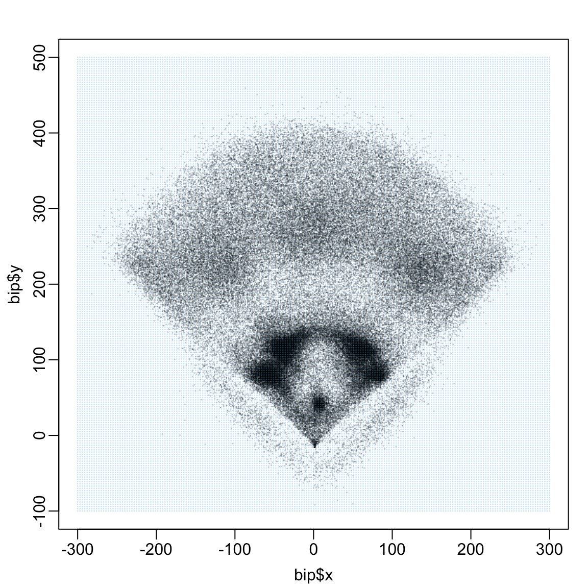
We will remove those (x,y) pairs in grid for which either
x + y < -100: these are locations far below the third base liney - x < -100: these are locations far below the first base linesqrt(x^2 +y^2 < 580): these are locations very far from home plate
grid <-
  raw_grid |>
  dplyr::filter(y + x > -100 & y - x > -100 & sqrt(x^2 + y^2) < 580)
plot(bip$x, bip$y,
     xlim = c(-300, 300), ylim = c(-100, 500),
     pch = 16, cex = 0.2,
     col = adjustcolor(oi_colors[1], alpha.f = 0.2))
points(grid$x, grid$y, pch = 16, cex = 0.2,
       col = adjustcolor(oi_colors[3], alpha.f = 0.3))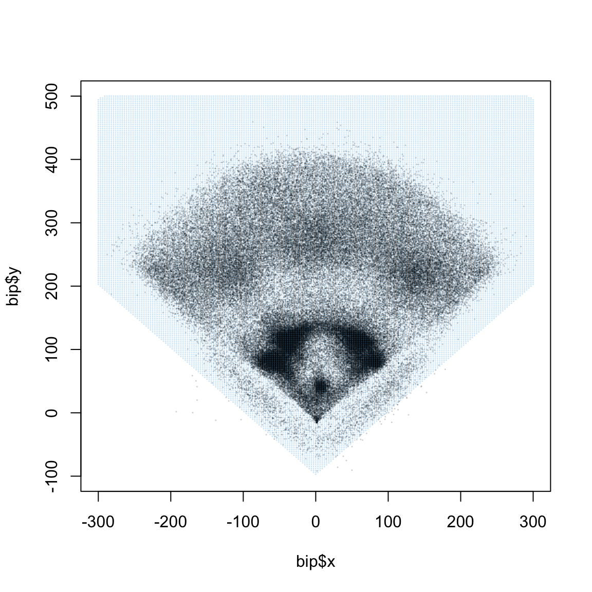
We can use the cut() function to divide the x and y values in bip into small bins. Here is a quick example of how cut works: we first create a vector with a few numbers. The breaks argument of cut tells it the end points of each bin.
x <- c(0.11, 0.23, 0.45, 0.67, 0.99, 0.02)
cut(x, breaks = seq(0, 1, by = 0.1))
[1] (0.1,0.2] (0.2,0.3] (0.4,0.5] (0.6,0.7] (0.9,1] (0,0.1]
10 Levels: (0,0.1] (0.1,0.2] (0.2,0.3] (0.3,0.4] (0.4,0.5] ... (0.9,1]Below, we first cut the values of x and y that appear in bip. Then, using a grouped summary, we can compute the number of balls hit to each bin and the proportion of those balls that result in an out.
bin_probs <-
bip |>
dplyr::select(x, y, Out) |>
dplyr::mutate(
x_bin = cut(x, breaks = seq(-300-grid_sep/2, 300+grid_sep/2, by = grid_sep)),
y_bin = cut(y, breaks = seq(-100 - grid_sep/2, 500+grid_sep/2, by = grid_sep))) |>
dplyr::group_by(x_bin, y_bin) |>
dplyr::summarise(
out_prob = mean(Out),
n_balls = dplyr::n(),
.groups = "drop")- 1
-
Offsetting by
grid_sep/2ensures that thexandyvalues ingridare the centers of the squares in our grid (and not one of the corners)
We can now bin the x and y values contained in grid and, using a left_join(), append a column that contains the estimated probability of an out hit to each 3ft x 3ft square in our grid. Note that if there is a combination of x_bin and y_bin in grid that is not contained in bin_prob, the estimated probability will be NA. These are grid squares in which no balls were hit.
grid_probs_bin <-
  grid |>
  dplyr::mutate(
    x_bin = cut(x, breaks = seq(-300-grid_sep/2, 300+grid_sep/2, by = 3)),
    y_bin = cut(y, breaks = seq(-100-grid_sep/2, 500+grid_sep/2, by = 3))) |>
  dplyr::left_join(y = bin_probs, by = c("x_bin", "y_bin"))
We can now make a heatmap of our estimated probabilities by looping over the rows in grid_prob_bins, drawing a small rectangle with corners (x-1.5, y-1.5), (x + 1.5, y-1.5), (x+1.5, y+1.5), and (x-1.5, y+1.5), and shading the rectangle based on the corresponding out probability.
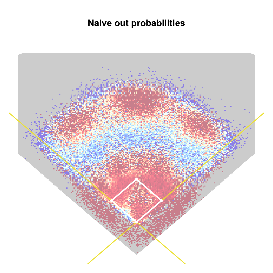
col_list <- colorBlindness::Blue2DarkRed18Steps
par(mar = c(1,1,5,1), mgp = c(1.8, 0.5, 0))
plot(1, type = "n",
xlim = c(-300, 300), ylim = c(-100, 500),
xaxt = "n", yaxt = "n", bty = "n",
main = "Naive out probabilities", xlab = "", ylab = "")
for(i in 1:nrow(grid_probs_bin)){
rect(xleft = grid_probs_bin$x[i] - grid_sep/2,
ybot = grid_probs_bin$y[i] - grid_sep/2,
xright = grid_probs_bin$x[i] + grid_sep/2,
ytop = grid_probs_bin$y[i] + grid_sep/2,
col = ifelse(
is.na(grid_probs_bin$out_prob[i]),
adjustcolor(oi_colors[1], alpha.f = 0.2),
adjustcolor(rgb(colorRamp(col_list,bias=1)(grid_probs_bin$out_prob[i])/255),
alpha.f = 0.5)),
border = NA)
}
abline(a = 0, b = 1, col = oi_colors[5], lwd = 2)
abline(a = 0, b = -1, col = oi_colors[5], lwd = 2)
lines(x = c(0,90/sqrt(2)), y = c(0, 90/sqrt(2)), col = "white", lwd = 3)
lines(x = c(0,-90/sqrt(2)), y = c(0, 90/sqrt(2)), col = "white", lwd = 3)
lines(x = c(90/sqrt(2), 0), y = c(90/sqrt(2), 90*sqrt(2)), col = "white", lwd = 3)
lines(x = c(-90/sqrt(2), 0), y = c(90/sqrt(2), 90*sqrt(2)), col = "white", lwd = 3)
points(x = 0, y = 0, pch = 16, cex = 0.8, col = "white")
points(x = 90/sqrt(2), y = 90/sqrt(2), pch = 16, cex = 0.8, col = "white")
points(x = -90/sqrt(2), y = 90/sqrt(2), pch = 16,cex = 0.8, col = "white")
points(x = 0, y = 90*sqrt(2), pch = 16, cex = 0.8, col = "white")- 1
- This is a popular diverging color palette, which ranges from blue to red, that is color-blind friendly. See here for more details.
- 2
-
Specifying
type = "n"tells R to make an empty plot - 3
- Manually set the horizontal and vertical limits of the plotting area
- 4
-
xaxt = "n"andyaxt = "n"suppress the axis lines andbty = "n"suppresses the bounding box - 5
-
maincontrols the title of plot while settingxlab = ""andylab = ""suppresses horizontal and vertical axis labels - 6
-
To use
rect(), we must pass the coordinates of the bottom left and top right corners of the rectangle - 7
- If there were no balls hit to a particular rectangle, we will color it gray. Otherwise, we will color it according to the fitted probability
- 8
-
The expression
rgb(colorRamp(col_list, bias=1)(grid_probs_bin$out_prob)/255)maps the fitted probability to a color incol_listusing linear interpolation. Here 0% maps to dark blue and 100% maps to dark red. - 9
- Suppresses the border of the rectangle
A Logistic Regression Model for Outs
Our naively estimated out probabilities leave much to be desired. For one thing, there are lots of “gaps” in the fitted surface where our initial model can’t make a prediction. These are the cells in our grid into which no balls were hit. Of much greater concern are the sharp discontinuities evident in the figure. In fact, there are many regions where the fitted out probability jumps from 0% to 100% to 0% in the span of about 6 feet. Such discontinuities are artifacts of the small sample sizes within some of the bins. Indeed, we find that about 85% of the grid cells contain 10 or fewer observations
mean(bin_probs$n_balls <= 10)[1] 0.8541364Like we did to predict XG using shot distance, we can overcome this challenge by building a statistical model. In particular, we would like to model the log-odds of an out as a function of the batted balls location. That is, \[ \log\left(\frac{\mathbb{P}(\textrm{out})}{1 - \mathbb{P}(\textrm{out})} \right) = s(x,y), \] where \(s\) is a smooth function of the batted balls location. What form should \(s\) take?
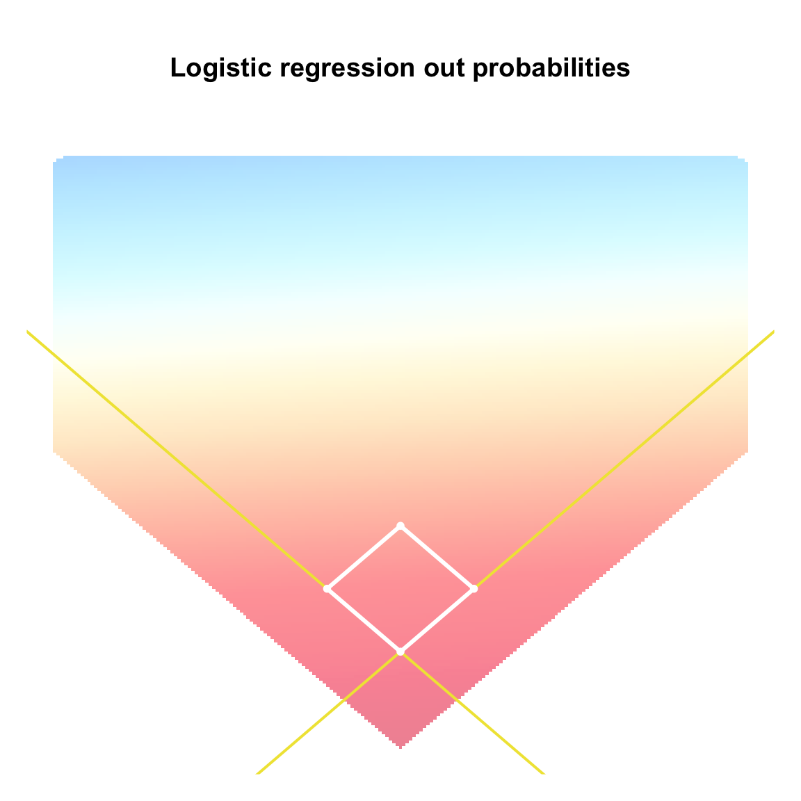
One possibility is to assume that there are parameters \(\beta_{0}, \beta_{x},\) and \(\beta_{y}\) such that \[
\log\left(\frac{\mathbb{P}(\textrm{out})}{1 - \mathbb{P}(\textrm{out})} \right) = \beta_{0} + \beta_{x}x + \beta_{y}y
\] We can estimate these parameters using glm() and then compute the fitted probability for every cell in our grid.
logit_fit <-
glm(Out ~ x + y,
family = binomial(link = "logit"), data = bip)
grid_logit_preds <-
predict(object = logit_fit,
newdata = grid, type = "response")
grid_logit_cols <-
rgb(colorRamp(col_list,bias=1)(grid_logit_preds)/255)- 1
-
To get fitted values on the probability scale, we need to specify
type = "response" - 2
- Creates a vector mapping the fitted probability at each grid location to a color between the two extremes
The fitted logistic regression model predicts that the probability of an out decreases as one moves vertically away from home plate. The model further predicts that balls hit into the outfield tend not to result in outs, which is at odds with what we see in the data. Indeed, our earlier plot revealed pockets of high out probability in the outfield, roughly corresponding to the usual positioning of the left, right, and center fielders.
par(mar = c(1,1,5,1), mgp = c(1.8, 0.5, 0))
plot(1, type = "n",
xlim = c(-300, 300), ylim = c(-100, 500),
xaxt = "n", yaxt = "n", bty = "n",
main = "Logistic regression out probabilities", xlab = "", ylab = "")
for(i in 1:nrow(grid_probs_bin)){
rect(xleft = grid_probs_bin$x[i] - grid_sep/2,
ybot = grid_probs_bin$y[i] - grid_sep/2,
xright = grid_probs_bin$x[i] + grid_sep/2,
ytop = grid_probs_bin$y[i] + grid_sep/2,
col = adjustcolor(grid_logit_cols[i], alpha.f = 0.5),
border = NA)
}
abline(a = 0, b = 1, col = oi_colors[5], lwd = 2)
abline(a = 0, b = -1, col = oi_colors[5], lwd = 2)
lines(x = c(0,90/sqrt(2)), y = c(0, 90/sqrt(2)), col = "white", lwd = 3)
lines(x = c(0,-90/sqrt(2)), y = c(0, 90/sqrt(2)), col = "white", lwd = 3)
lines(x = c(90/sqrt(2), 0), y = c(90/sqrt(2), 90*sqrt(2)), col = "white", lwd = 3)
lines(x = c(-90/sqrt(2), 0), y = c(90/sqrt(2), 90*sqrt(2)), col = "white", lwd = 3)
points(x = 0, y = 0, pch = 16, cex = 0.8, col = "white")
points(x = 90/sqrt(2), y = 90/sqrt(2), pch = 16, cex = 0.8, col = "white")
points(x = -90/sqrt(2), y = 90/sqrt(2), pch = 16,cex = 0.8, col = "white")
points(x = 0, y = 90*sqrt(2), pch = 16, cex = 0.8, col = "white")- 1
-
Unlike with binning-and-averaging, our parametric model is able to make predictions at grid cells not present in the training data. So, we don’t need to check whether the predicted probability is
NA
Generalized Additive Models
The root cause of the conflict between our data and the logistic regression model forecasts in Figure 7 is the model’s strong — and totally unrealistic — assumption that the log-odds of an out is linear in both \(x\) and \(y.\) A more accurate model would allow the log-odds to vary non-linearly.
Generalized Additive Models (or GAMs) are an elegant way to introduce non-linearity and create spatially smooth maps. In our context, a GAM model expresses \(s(x,y)\) as a linear combination of a large number of two-dimensional splines functions. Each spline function is a piecewise polynomial that is localized to a small region of \((x,y)\) space, meaning that it is non-zero inside the region and zero outside the region. Such spline functions can be linearly combined to approximate really complicated functions arbitrarily well2
We can fit GAMs in R using the mgcv package, which can be installed using
install.packages("mgcv")The package provides two fitting functions, gam() and bam(), which is recommended for very large data sets like bip. Both functions are similar lm() and glm() in that they require users to specify a formula and, in the case of non-continuous outcomes, a link function. The main difference is the term s(), which is used to signal to gam() or bam() that we want to smooth over whatever variables appear inside of the brackets of s(). In our case, because we wish to smooth over both x and y, we will include the terms s(x,y)
Warning
Fitting our out probability model takes a few minutes
library(mgcv)
gam_fit <-
  bam(formula = Out ~ s(x,y),
      family = binomial(link="logit"), data = bip)
After fitting our GAM, we can visualize the estimated out probabilities:
grid_gam_preds <-
  predict(object = gam_fit,
          newdata = grid, type = "response")

grid_gam_cols <-
  rgb(colorRamp(col_list,bias=1)(grid_gam_preds)/255)

par(mar = c(1,1,5,1), mgp = c(1.8, 0.5, 0))
plot(1, type = "n",
     xlim = c(-300, 300), ylim = c(-100, 500),
     xaxt = "n", yaxt = "n", bty = "n",
     main = "GAM out probabilities", xlab = "", ylab = "")

for(i in 1:nrow(grid_probs_bin)){
  rect(xleft = grid_probs_bin$x[i] - grid_sep/2,
       ybot = grid_probs_bin$y[i] - grid_sep/2,
       xright = grid_probs_bin$x[i] + grid_sep/2,
       ytop = grid_probs_bin$y[i] + grid_sep/2,
       col = adjustcolor(grid_gam_cols[i], alpha.f = 0.5),
       border = NA)
}
abline(a = 0, b = 1, col = oi_colors[5], lwd = 2)
abline(a = 0, b = -1, col = oi_colors[5], lwd = 2)

lines(x = c(0,90/sqrt(2)), y = c(0, 90/sqrt(2)), col = "white", lwd = 3)
lines(x = c(0,-90/sqrt(2)), y = c(0, 90/sqrt(2)), col = "white", lwd = 3)
lines(x = c(90/sqrt(2), 0), y = c(90/sqrt(2), 90*sqrt(2)), col = "white", lwd = 3)
lines(x = c(-90/sqrt(2), 0), y = c(90/sqrt(2), 90*sqrt(2)), col = "white", lwd = 3)


points(x = 0, y = 0, pch = 16, cex = 0.8, col = "white")
points(x = 90/sqrt(2), y = 90/sqrt(2), pch = 16, cex = 0.8, col = "white")
points(x = -90/sqrt(2), y = 90/sqrt(2), pch = 16,cex = 0.8, col = "white")
points(x = 0, y = 90*sqrt(2), pch = 16, cex = 0.8, col = "white")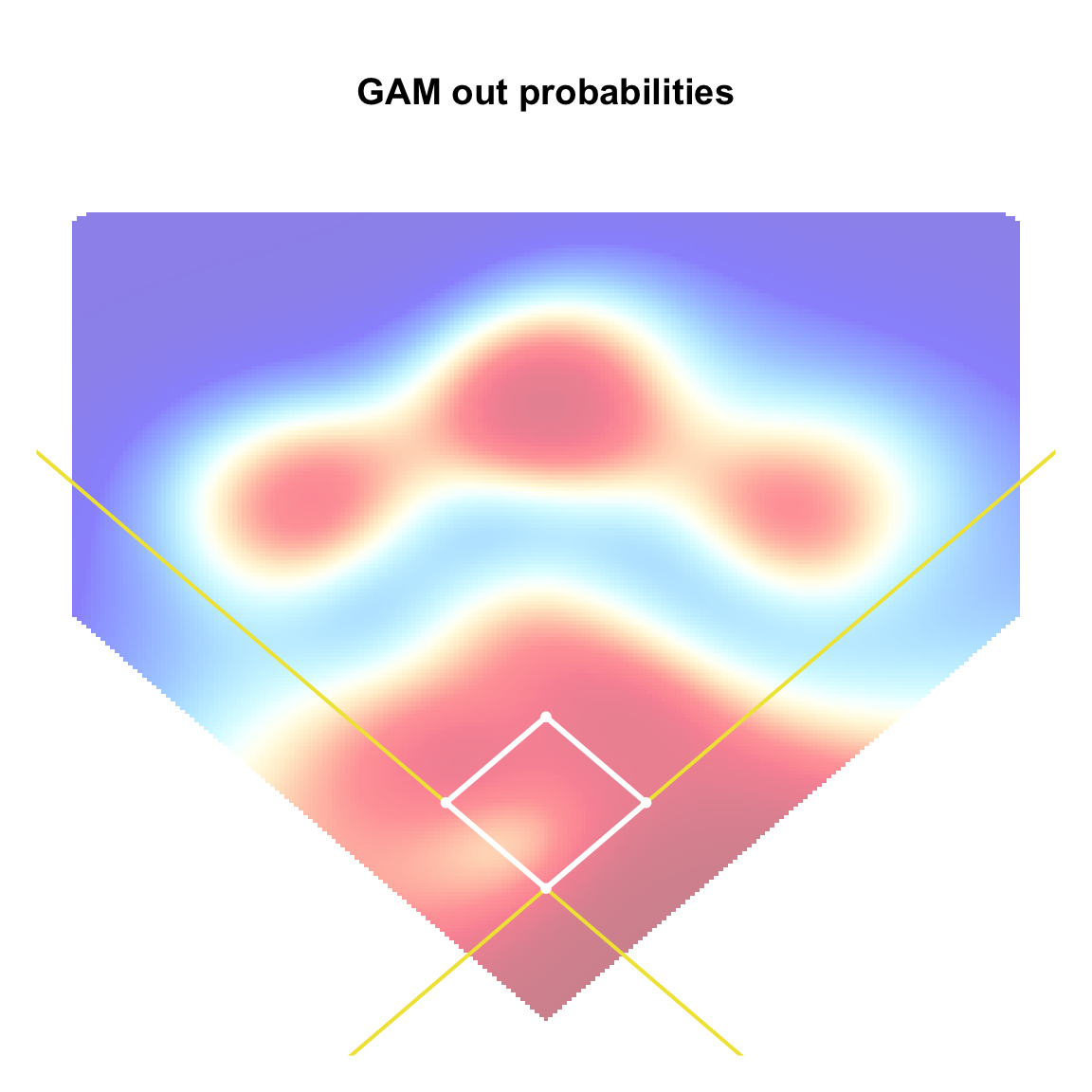
The out probabilities fitted by the GAM appear much more reasonable: balls hit within the in-field and close to the outfielders tend to be result in outs while balls hit in the gap between the infield and outfield tend not to result in outs.
Dividing Defensive Run Value
Recall that if at-bat \(i\) results in a ball put in play, we will distribute \(\delta_{i}^{(f)} = -\delta_{i} \times \hat{p}_{i}\) to the fielders and assign \(\delta_{i}^{(p)} = -\delta \times (1 - \hat{p}_{i})\) to the pitcher. The following code adds a column to def_atbat2024 containing the predicted out probabilities from our fitted GAM. Note that this column contains NA values for those at-bats that did not result in a ball in play (e.g., they ended with a walk or a strikeout or a home run) For the vast majority of these at-bats, we will manually set \(\hat{p}_{i} = 0\) so that the pitcher gets all the credit (i.e., \(\delta^{(p)}_{i} = -\delta_{i}\)).
all_preds <-
predict(object = gam_fit,
newdata = def_atbat2024,
type = "response")
def_atbat2024$p_out <- all_preds
def_atbat2024 <-
def_atbat2024 |>
dplyr::mutate(
p_out = dplyr::case_when(
is.na(p_out) & end_events == "home_run" ~ 0,
is.na(p_out) & end_type != "X" ~ 0,
.default = p_out))- 1
-
When
xandyareNA(i.e., whenever the at-bat doesn’t end with a ball in play),predictwill returnNA. - 2
- Adds fitted out probabilities to the data table
- 3
-
For home runs, manually set
p_out = 0(so pitcher gets all credit/blame) - 4
-
For at-bats that end with a ball or strike, set
p_out = 0(so pitcher gets all credit/blame)
Even after manually setting \(\hat{p}_{i} = 0\) on the at-bats that didn’t end with the ball in play, there are still some NA values in the column p_out. On further inspection, it looks like these were at-bats in which the ball was put in play but are missing hit locations.
table(def_atbat2024$end_events[is.na(def_atbat2024$p_out)])
                   double                 field_out grounded_into_double_play
                        2                         5                         1
                   single                    triple
4 1 sum(is.na(def_atbat2024$x[is.na(def_atbat2024$p_out)]))[1] 13We will remove these rows from our calculations
def_atbat2024 <-
  def_atbat2024 |>
  dplyr::filter(!is.na(p_out))
We can now finally compute \(\delta^{(f)}_{i}\) and \(\delta^{(p)}_{i}\) for each at-bat.
def_atbat2024 <-
  def_atbat2024 |>
  dplyr::mutate(
    delta_p = -1 * (1 - p_out) * RunValue,
    delta_f = -1 * p_out * RunValue)
Fielding Run Values
If a ball is hit towards deep left field and results in the fielding team creating a large \(-\delta\), how much blame should the third baseman, who is on the opposite side of the park receive? Following Baumer, Jensen, and Matthews (2015), we will apportion \(\delta_{i}^{(f)},\) the portion of the run value \(-\delta_{i}\) attributable to the fielding in at-bat \(i\), based on each fielder’s responsibility for making an out on the batted ball. Specifically, we will assign \(w_{i,\ell} \times \delta_{i}^{(f)}\) to the fielder playing position \(\ell \in \{1, 2, \ldots, 9\}\) during the at-bat where \[ w_{i,\ell} = \frac{\hat{p}_{i,\ell}}{\hat{p}_{i,1} + \cdots + \hat{p}_{i,9}} \] and \(\hat{p}_{i,\ell}\) is the probability that fielder \(\ell\) makes the out given the location of the batted ball.
To estimate the \(\hat{p}_{i,\ell}\)’s, we will fit 9 separate GAMs, one for each fielding position. For fielding position \(\ell,\) we will create a new variable that is equal to 1 if the ball in play resulted in an out was initially fielded by the player at position \(\ell.\) Unlike our overall out probability model, which we fit using data from all batted balls, each position-specific GAM will be fitted using data from the subset of batted balls that are reasonably close to the typical position location. For instance, when fitting the model for the first basemen, we won’t include data from balls hit into deep left field. We compute the coordinates of the typical position by taking the average value of the x and y coordinates of all batted balls fielded by players at position \(\ell.\) We fit each position-specific GAM using batted balls hit within 150 ft of this typical location3
Warning
This code takes between several minutes to run
mid_x <- rep(NA, times = 9)
mid_y <- rep(NA, times = 9)
fit_list <- list()
fit_time <- rep(NA, times = 9)
for(l in 1:9){
print(paste0("Starting l = ", Sys.time()))
mid_x[l] <- mean(bip$x[bip$end_hit_location == l], na.rm = TRUE)
mid_y[l] <- mean(bip$y[bip$end_hit_location==l], na.rm = TRUE)
train_df <-
bip |>
dplyr::mutate(newOut = ifelse(Out == 1 & end_hit_location == l, 1, 0)) |>
dplyr::filter(!is.na(x) & !is.na(y)) |>
dplyr::filter( sqrt( (x - mid_x[l])^2 + (y - mid_y[l])^2 ) < 150) |>
dplyr::select(x,y,newOut)
fit_time[l] <-
system.time(
fit_list[[l]] <-
bam(formula = newOut ~ s(x, y),
family = binomial(link="logit"),data = train_df))["elapsed"]
tmp_df <-
def_atbat2024 |>
dplyr::mutate(
x = ifelse(sqrt( (x - mid_x[l])^2 + (y - mid_y[l])^2 ) < 150, x, NA),
y = ifelse(sqrt( (x - mid_x[l])^2 + (y - mid_y[l])^2 ) < 150, y, NA)
)
preds <- predict(object = fit_list[[l]], newdata = tmp_df, type = "response")
def_atbat2024[[paste0("p_out_", l)]] <- preds
}
save(fit_list, mid_x, mid_y, file = "position_gam_fits.RData")- 1
- Vectors containing coordinates for the typical fielder location
- 2
- Holds all fitted objects, so that we can use them later to visualize position-specific out probabilities
- 3
-
Compute typical coordinates for position
l - 4
- Create position-specific outcome variable
- 5
- Subsets to batted balls within 150 ft of the typical location
- 6
-
It’s often helpful to track how long it takes to fit a model.
system.time()can return, among other things, the elapsed time. We save the time for fitting each position’s model in the vectorfit_time - 7
-
Instead of creating a different object for each position’s fitted model, we will store all the fitted models in a single
list, which can be saved. - 8
-
system.time()returns three different time measures. The most pertinent one is the actual elapsed time, stored in the slot “elapsed”. - 9
-
We only want model predictions for balls hit within 150ft of the typical location. Passing
NAxandyvalues topredict()is a hack to suppress model predictions for balls hit outside this radius. We will later over-write the resultingNA’s with 0’s. - 10
-
fit_list[[l]]is the fitted object return bybamfor positionl. - 11
-
Creates a column in
def_atbat2024holding the - 12
- Save’s the list containing all position-specific fits
[1] "Starting l = 2025-09-15 15:02:35.997148"
[1] "Starting l = 2025-09-15 15:03:50.958322"
[1] "Starting l = 2025-09-15 15:05:01.716077"
[1] "Starting l = 2025-09-15 15:06:28.180436"
[1] "Starting l = 2025-09-15 15:07:55.643024"
[1] "Starting l = 2025-09-15 15:09:18.325996"
[1] "Starting l = 2025-09-15 15:10:39.797597"
[1] "Starting l = 2025-09-15 15:11:20.999067"
[1] "Starting l = 2025-09-15 15:12:01.75346"
The columns p_out_1, …, p_out_9 in def_atbat2024 contain several NA values. Some of these correspond to at-bats that did not result in ball being put in play (i.e., those with end_type = S or end_type = B) while others correspond to at-bats in which the ball was hit far away from the typical location of the fielder. For these latter at-bats, we will manually set the position-specific out probabilities as follows: 1. For home runs and balls hit outside the 150ft radius for each position, we set p_out_* = 0 2. For at-bats ending with a strike or ball, we keep p_out_* = NA. 3. For balls in play with missing x and y coordinates, we set p_out_* = NA
Code
def_atbat2024 <-
  def_atbat2024 |>
  dplyr::mutate(
    p_out_1 = dplyr::case_when(
      end_events == "home_run" ~ 0,
      end_type %in% c("S", "B") ~ NA,
      is.na(x) | is.na(y) ~ NA,
      sqrt( (x - mid_x[1])^2 + (y - mid_y[1])^2) >= 150 ~ 0,
      .default = p_out_1),
    p_out_2 = dplyr::case_when(
      end_events == "home_run" ~ 0,
      end_type %in% c("S", "B") ~ NA,
      is.na(x) | is.na(y) ~ NA,
      sqrt( (x - mid_x[2])^2 + (y - mid_y[2])^2) >= 150 ~ 0,
      .default = p_out_2),
    p_out_3 = dplyr::case_when(
      end_events == "home_run" ~ 0,
      end_type %in% c("S", "B") ~ NA,
      is.na(x) | is.na(y) ~ NA,
      sqrt( (x - mid_x[3])^2 + (y - mid_y[3])^2) >= 150 ~ 0,
      .default = p_out_3),
    p_out_4 = dplyr::case_when(
      end_events == "home_run" ~ 0,
      end_type %in% c("S", "B") ~ NA,
      is.na(x) | is.na(y) ~ NA,
      sqrt( (x - mid_x[4])^2 + (y - mid_y[4])^2) >= 150 ~ 0,
      .default = p_out_4),
    p_out_5 = dplyr::case_when(
      end_events == "home_run" ~ 0,
      end_type %in% c("S", "B") ~ NA,
      is.na(x) | is.na(y) ~ NA,
      sqrt( (x - mid_x[5])^2 + (y - mid_y[5])^2) >= 150 ~ 0,
      .default = p_out_5),
    p_out_6 = dplyr::case_when(
      end_events == "home_run" ~ 0,
      end_type %in% c("S", "B") ~ NA,
      is.na(x) | is.na(y) ~ NA,
      sqrt( (x - mid_x[6])^2 + (y - mid_y[6])^2) >= 150 ~ 0,
      .default = p_out_6),
    p_out_7 = dplyr::case_when(
      end_events == "home_run" ~ 0,
      end_type %in% c("S", "B") ~ NA,
      is.na(x) | is.na(y) ~ NA,
      sqrt( (x - mid_x[7])^2 + (y - mid_y[7])^2) >= 150 ~ 0,
      .default = p_out_7),
    p_out_8 = dplyr::case_when(
      end_events == "home_run" ~ 0,
      end_type %in% c("S", "B") ~ NA,
      is.na(x) | is.na(y) ~ NA,
      sqrt( (x - mid_x[8])^2 + (y - mid_y[8])^2) >= 150 ~ 0,
      .default = p_out_8),
    p_out_9 = dplyr::case_when(
      end_events == "home_run" ~ 0,
      end_type %in% c("S", "B") ~ NA,
      is.na(x) | is.na(y) ~ NA,
      sqrt( (x - mid_x[9])^2 + (y - mid_y[9])^2) >= 150 ~ 0,
      .default = p_out_9))
We now normalize the \(\hat{p}_{i,\ell}\) values to get the weights \(w_{i,\ell}\) measuring the responsibility of each fielder for making an out in the at-bat.
def_atbat2024 <-
  def_atbat2024 |>
  dplyr::mutate(
    total_weight = p_out_1 + p_out_2 + p_out_3 +
      p_out_4 + p_out_5 + p_out_6 +
      p_out_7 + p_out_8 + p_out_9,
    w1 = p_out_1/total_weight,
    w2 = p_out_2/total_weight,
    w3 = p_out_3/total_weight,
    w4 = p_out_4/total_weight,
    w5 = p_out_5/total_weight,
    w6 = p_out_6/total_weight,
    w7 = p_out_7/total_weight,
    w8 = p_out_8/total_weight,
    w9 = p_out_9/total_weight)
Now, for each fielding position, we can compute \(w_{i,\ell} \times \delta^{(f)}_{i}\) and aggregate these values across players at that position to compute \(\textrm{RAA}_{\ell}^{(f)},\) which quantifies the total run value created by the player through their fielding at position \(\ell.\) Negative values of \(\textrm{RAA}_{\ell}^{(f)}\) suggest that the player’s fielding at position \(\ell\) netted positive run value for the batting team, thereby negatively impacthing his own team.
Here is the calculation for first basemen (fielding position number \(\ell = 3\)). Taking a looking at the largest \(\textrm{RAA}_{\ell}^{f}\) values, we see several recent Golden Glove winners who are known for their fielding prowess (Santana, Walker, Goldschmidt, Olson, Guerrero).
raa_f3 <-
  def_atbat2024 |>
  dplyr::mutate(RAA_f3 = delta_f * w3) |>
  dplyr::group_by(fielder_3) |>
  dplyr::summarize(RAA_f3 = sum(RAA_f3, na.rm = TRUE)) |>
  dplyr::rename(key_mlbam = fielder_3)

raa_f3 |>
  dplyr::inner_join(y = player2024_lookup, by = "key_mlbam") |>
  dplyr::select(Name, RAA_f3) |>
  dplyr::arrange(dplyr::desc(RAA_f3)) |>
  dplyr::slice_head(n = 10)
# A tibble: 10 × 2
Name RAA_f3
<chr> <dbl>
1 Carlos Santana 55.7
2 Christian Walker 54.6
3 Paul Goldschmidt 52.4
4 Bryce Harper 51.1
5 Matt Olson 51.0
6 Ryan Mountcastle 48.7
7 Vladimir Guerrero 47.1
8 Michael Toglia 46.5
9 Freddie Freeman 46.2
10 Josh Naylor 46.2The following code repeats this calculation for all fielding positions.
Show the code computes the fielding RAA for all positions.
raa_f1 <-
  def_atbat2024 |>
  dplyr::mutate(RAA_f1 = delta_f * w1) |>
  dplyr::group_by(pitcher) |>
  dplyr::summarize(RAA_f1 = sum(RAA_f1, na.rm = TRUE)) |>
  dplyr::rename(key_mlbam = pitcher) |>
  dplyr::select(key_mlbam, RAA_f1)

raa_f2 <-
  def_atbat2024 |>
  dplyr::mutate(RAA_f2 = delta_f * w2) |>
  dplyr::group_by(fielder_2) |>
  dplyr::summarize(RAA_f2 = sum(RAA_f2, na.rm = TRUE)) |>
  dplyr::rename(key_mlbam = fielder_2) |>
  dplyr::select(key_mlbam, RAA_f2)

raa_f3 <-
  def_atbat2024 |>
  dplyr::mutate(RAA_f3 = delta_f * w3) |>
  dplyr::group_by(fielder_3) |>
  dplyr::summarize(RAA_f3 = sum(RAA_f3, na.rm = TRUE)) |>
  dplyr::rename(key_mlbam = fielder_3) |>
  dplyr::select(key_mlbam, RAA_f3)

raa_f4 <-
  def_atbat2024 |>
  dplyr::mutate(RAA_f4 = delta_f * w4) |>
  dplyr::group_by(fielder_4) |>
  dplyr::summarize(RAA_f4 = sum(RAA_f4, na.rm = TRUE)) |>
  dplyr::rename(key_mlbam = fielder_4) |>
  dplyr::select(key_mlbam, RAA_f4)

raa_f5 <-
  def_atbat2024 |>
  dplyr::mutate(RAA_f5 = delta_f * w5) |>
  dplyr::group_by(fielder_5) |>
  dplyr::summarize(RAA_f5 = sum(RAA_f5, na.rm = TRUE)) |>
  dplyr::rename(key_mlbam = fielder_5) |>
  dplyr::select(key_mlbam, RAA_f5)

raa_f6 <-
  def_atbat2024 |>
  dplyr::mutate(RAA_f6 = delta_f * w6) |>
  dplyr::group_by(fielder_6) |>
  dplyr::summarize(RAA_f6 = sum(RAA_f6, na.rm = TRUE)) |>
  dplyr::rename(key_mlbam = fielder_6) |>
  dplyr::select(key_mlbam, RAA_f6)

raa_f7 <-
  def_atbat2024 |>
  dplyr::mutate(RAA_f7 = delta_f * w7) |>
  dplyr::group_by(fielder_7) |>
  dplyr::summarize(RAA_f7 = sum(RAA_f7, na.rm = TRUE)) |>
  dplyr::rename(key_mlbam = fielder_7) |>
  dplyr::select(key_mlbam, RAA_f7)

raa_f8 <-
  def_atbat2024 |>
  dplyr::mutate(RAA_f8 = delta_f * w8) |>
  dplyr::group_by(fielder_8) |>
  dplyr::summarize(RAA_f8 = sum(RAA_f8, na.rm = TRUE)) |>
  dplyr::rename(key_mlbam = fielder_8) |>
  dplyr::select(key_mlbam, RAA_f8)

raa_f9 <-
  def_atbat2024 |>
  dplyr::mutate(RAA_f9 = delta_f * w9) |>
  dplyr::group_by(fielder_9) |>
  dplyr::summarize(RAA_f9 = sum(RAA_f9, na.rm = TRUE)) |>
  dplyr::rename(key_mlbam = fielder_9) |>
  dplyr::select(key_mlbam, RAA_f9)
Like we did when computing \(\textrm{RAA}^{(br)}\) in Lecture 7, we will concatenate raa_f1, …, raa_f9 and sum every players total contributions across all fielding positions.
raa_f <-
  raa_f1 |>
  dplyr::full_join(y = raa_f2, by = "key_mlbam") |>
  dplyr::full_join(y = raa_f3, by = "key_mlbam") |>
  dplyr::full_join(y = raa_f4, by = "key_mlbam") |>
  dplyr::full_join(y = raa_f5, by = "key_mlbam") |>
  dplyr::full_join(y = raa_f6, by = "key_mlbam") |>
  dplyr::full_join(y = raa_f7, by = "key_mlbam") |>
  dplyr::full_join(y = raa_f8, by = "key_mlbam") |>
  dplyr::full_join(y = raa_f9, by = "key_mlbam") |>
  tidyr::replace_na(
    list(RAA_f1=0, RAA_f2=0, RAA_f3=0, RAA_f4=0,
         RAA_f5=0, RAA_f6 = 0, RAA_f7=0, RAA_f8 = 0, RAA_f9=0)) |>
  dplyr::mutate(
    RAA_f = RAA_f1 + RAA_f2 + RAA_f3 + RAA_f4 +
      RAA_f5 + RAA_f6 + RAA_f7 + RAA_f8 + RAA_f9) |>
  dplyr::inner_join(y = player2024_lookup, by = "key_mlbam") |>
  dplyr::select(Name, key_mlbam, RAA_f, RAA_f1, RAA_f2, RAA_f3, RAA_f4, RAA_f5,
                RAA_f6, RAA_f7, RAA_f8, RAA_f9)
Pitching Run Values
Recall that \(\delta_{i}^{(p)}\) is the amount of run value created by the pitcher in at-bat \(i.\) Summing this value across all at-bats involving each pitcher, we obtain each pitchers \(\textrm{RAA}^{(p)}.\)
raa_p <-
  def_atbat2024 |>
  dplyr::select(pitcher, delta_p) |>
  dplyr::group_by(pitcher) |>
  dplyr::summarise(RAA_p = sum(delta_p, na.rm = TRUE)) |>
  dplyr::rename(key_mlbam = pitcher) |>
  dplyr::inner_join(y = player2024_lookup, by = "key_mlbam") |>
  dplyr::select(Name, key_mlbam, RAA_p)
We see that the two 2024 Cy Young Award winners4, Tarik Skubal and Chris Sale, have the highest \(\textrm{RAA}^{(p)}\) values.
raa_p |>
  dplyr::arrange(dplyr::desc(RAA_p)) |>
  dplyr::slice_head(n=10)
# A tibble: 10 × 3
Name key_mlbam RAA_p
<chr> <int> <dbl>
1 Tarik Skubal 669373 14.7
2 Chris Sale 519242 14.6
3 Ryan Walker 676254 13.5
4 Cade Smith 671922 13.3
5 Paul Skenes 694973 12.3
6 Emmanuel Clase 661403 11.2
7 Kirby Yates 489446 9.99
8 Griffin Jax 643377 9.53
9 Edwin Uceta 670955 9.23
10 Garrett Crochet 676979 9.13We will save both raa_f and raa_p for later use
save(raa_f, raa_p, file = "raa_defensive2024.RData")Replacement Level
We now combine the fielding and pitching RAA values with the baserunning and batting RAA values we computed in Lecture 7 into a single table.
load("raa_offensive2024.RData")

raa <-
  raa_b |>
  dplyr::select(-Name) |>
  dplyr::full_join(y = raa_br |> dplyr::select(-Name), by = "key_mlbam") |>
  dplyr::full_join(y = raa_p |> dplyr::select(-Name), by = "key_mlbam") |>
  dplyr::full_join(y = raa_f |> dplyr::select(-Name), by = "key_mlbam") |>
  tidyr::replace_na(list(RAA_b = 0, RAA_br = 0, RAA_f = 0, RAA_p = 0)) |>
  dplyr::mutate(RAA = RAA_b + RAA_br + RAA_f + RAA_p) |>
  dplyr::left_join(y = player2024_lookup |> dplyr::select(key_mlbam, Name), by = "key_mlbam") |>
  dplyr::select(Name, key_mlbam, RAA, RAA_b, RAA_br, RAA_f, RAA_p)
\(RAA\) is a comprehensive measure of a player’s performance that accounts not only for the actual runs scored (or given up) due to his contributions but also the changes in the expected runs that can be attributed to his play. We constructed \(RAA\) so that larger numbers indicate better performance. While the absolute \(RAA\) values are useful on their own, they become even more useful — and easier to interpret — when calibrated to measure performance relative to a baseline player. As argued by Baumer, Jensen, and Matthews (2015), although comparing an individual players \(RAA\) to the league-average value is intuitive, average players are themselves quite valuable. Further, it is not reasonable to expect a team to be able to replace any player with a league average one. Thus, it is more useful to compare each player’s performance relative to a replacement-level player.
As discussed in class (and also in (Baumer, Jensen, and Matthews 2015, sec. 3.8)), existing definitions of replacement level are fairly arbitrary. For instance, back in 2010, FanGraphs asserted that a team of players making the minimum MLB salary would win 29.7% of its games (so between 48 and 49 games). Similar definitions have been adopted by other sites like Baseball Propsectus and Baseball Reference. Unfortunately, there is little empirical justification for this number.
We will instead use Baumer, Jensen, and Matthews (2015)’s roster-based definition of replacement level, which is motivated and computed as follows:
- Each of the 30 major league teams typically carries 25 players, 13 of whom are position players and 12 of whom are pitchers
- On any given day, there are generally \(12 \times 30 = 360\) pitchers and \(13 \times 30 = 390\) active players.
- So, we will treat the 390 position players with the most plate appearances and the 360 pitchers who faced the most batters as non-replacement level and everyone else as replacement-level.
Remember that our table def_atbat2024 contains information from all available at-bats in the 2024 regular season. We can use the data in this table to count the number of plate appearances for each non-pitcher and number of batters faced by each pitcher. To this end, we first create lists of the MLB Advanced Media IDs of all pitchers and all non-pitchers who appear in our dataset.
all_players <- unique(
c(def_atbat2024$batter, def_atbat2024$pitcher, def_atbat2024$fielder_2,
def_atbat2024$fielder_3, def_atbat2024$fielder_4, def_atbat2024$fielder_5,
def_atbat2024$fielder_6, def_atbat2024$fielder_7, def_atbat2024$fielder_8, def_atbat2024$fielder_9))
pitchers <- unique(def_atbat2024$pitcher)
position_players <- all_players[!all_players %in% pitchers]- 1
- Get the ID for all players
- 2
- Get the ID for all pitchers
- 3
- Pull out the ID for all non-pitchers
Using grouped summaries, we can count the number of at-bats faced by each position player as a batter and by each pitcher. Since the overwhelming majority of at-bats involved only one batter, these counts effectively tell us the number of batters faced by each pitcher.
position_pa <-
def_atbat2024 |>
dplyr::filter(batter %in% position_players) |>
dplyr::group_by(batter) |>
dplyr::summarise(n = dplyr::n()) |>
dplyr::arrange(dplyr::desc(n)) |>
dplyr::rename(key_mlbam = batter)
pitcher_pa <-
def_atbat2024 |>
dplyr::group_by(pitcher) |>
dplyr::summarise(n = dplyr::n()) |>
dplyr::arrange(dplyr::desc(n)) |>
dplyr::rename(key_mlbam = pitcher)
repl_position_players <- position_pa$key_mlbam[-(1:390)]
repl_pitchers <- pitcher_pa$key_mlbam[-(1:360)]
cat("Cut-off for position players:", position_pa$n[390], "\n")
cat("Cut-off for pitchers:", pitcher_pa$n[360], "\n")- 1
- This removes at-bats in which a pitcher is hitting
- 2
- Counts the number of at-bats in which each position player is batting
- 3
- Arranges the counts in decreasing order so that we can determine replacement-level cut-offs
- 4
-
Since the vector
pitchersis just the unique values ofdef_atbat2024$pitcher, there is no need to filter - 5
- Get the IDs of the position players and pitchers outside, respectively, the top 390 and 360 numbers of plate appearances
Cut-off for position players: 131
Cut-off for pitchers: 204
Ultimately, we wish to compare each player’s \(RAA\) to the \(RAA\) that would have been created had the player been replaced by a replacement-level player. To estimate this counter-factual \(RAA\), we will divide the total \(RAA\) produced by all replacement-level players by the total number of plate appearances.
repl_position_raa <-
raa |>
dplyr::filter(key_mlbam %in% repl_position_players) |>
dplyr::inner_join(y = position_pa, by = "key_mlbam") |>
dplyr::select(Name, key_mlbam, RAA, n)
repl_pitch_raa <-
raa |>
dplyr::filter(key_mlbam %in% repl_pitchers) |>
dplyr::inner_join(y = pitcher_pa, by = "key_mlbam") |>
dplyr::select(Name, key_mlbam, RAA, n)
repl_avg_pos <- sum(repl_position_raa$RAA)/sum(repl_position_raa$n)
repl_avg_pitch <- sum(repl_pitch_raa$RAA)/sum(repl_pitch_raa$n)- 1
-
Using an inner join ensures that we only append the
nvalues for replacement-level players
We see that the replacement-level RAA per-at-bat is 0 for position players and -0.02 for pitchers. Multiplying the the replacement-level per-at-bat RAA values by the number of plate appearances faced by each non-replacement-level player gives us an estimate of how each player’s replacement-level “shadow” would perform. Finally, using the heuristic of 10 runs per win, dividing the difference between the actual RAA and the RAA for the replacement-level shadow yields our wins above replacement for position players.
position_war <-
  raa |>
  dplyr::filter(!key_mlbam %in% repl_position_players) |>
  dplyr::inner_join(y = position_pa, by = "key_mlbam") |>
  dplyr::select(Name, key_mlbam, RAA, n) |>
  dplyr::mutate(shadowRAA = n * repl_avg_pos) |>
  dplyr::mutate(WAR = (RAA - shadowRAA)/10)

position_war |>
  dplyr::arrange(dplyr::desc(WAR)) |>
  dplyr::slice_head(n = 10)
# A tibble: 10 × 6
Name key_mlbam RAA n shadowRAA WAR
<chr> <dbl> <dbl> <int> <dbl> <dbl>
1 Bobby Witt 677951 165. 694 -1.36 16.6
2 Gunnar Henderson 683002 117. 702 -1.37 11.8
3 Elly De La Cruz 682829 114. 679 -1.33 11.5
4 Jose Ramirez 608070 113. 657 -1.28 11.5
5 Zach Neto 687263 110. 590 -1.15 11.1
6 Marcus Semien 543760 108. 701 -1.37 10.9
7 Ketel Marte 606466 101. 562 -1.10 10.2
8 Vladimir Guerrero 665489 99.0 671 -1.31 10.0
9 Francisco Lindor 596019 98.5 689 -1.35 9.98
10 Jose Altuve 514888 98.2 661 -1.29 9.95We can run a similar calculation for pitchers.
pitch_war <-
  raa |>
  dplyr::filter(!key_mlbam %in% repl_pitchers) |>
  dplyr::inner_join(y = pitcher_pa, by = "key_mlbam") |>
  dplyr::select(Name, key_mlbam, RAA, n) |>
  dplyr::mutate(shadowRAA = n * repl_avg_pitch) |>
  dplyr::mutate(WAR = (RAA - shadowRAA)/10)

pitch_war |>
  dplyr::arrange(dplyr::desc(WAR)) |>
  dplyr::slice_head(n = 10)
# A tibble: 10 × 6
Name key_mlbam RAA n shadowRAA WAR
<chr> <dbl> <dbl> <int> <dbl> <dbl>
1 Tarik Skubal 669373 17.2 730 -17.7 3.49
2 Chris Sale 519242 17.2 702 -17.0 3.42
3 Zack Wheeler 554430 10.1 759 -18.4 2.86
4 Paul Skenes 694973 14.6 495 -12.0 2.66
5 Garrett Crochet 676979 9.91 596 -14.5 2.44
6 Bryce Miller 682243 7.66 681 -16.5 2.42
7 Seth Lugo 607625 2.47 813 -19.7 2.22
8 Ryan Walker 676254 14.7 302 -7.33 2.21
9 Reynaldo Lopez 625643 8.82 542 -13.2 2.20
10 Cade Smith 671922 14.2 289 -7.02 2.12Exercises
- We modeled the probability of a batted ball resulting in out using just the batted ball location. Try adjusting for additional factors about the pitch and swing in our GAM. How do the out probabilities and our downstream analysis change when you account for these factors?
References
Baumer, Benjamin S., Shane T. Jensen, and Gregory J. Matthews. 2015. “openWAR: An Open Source System for Evaluating Overall Player Performance in Major League Baseball.” Journal of Quantitative Analysis in Sports 11 (2).
Footnotes
The official position numbers are: 1 (pitcher), 2 (catcher), 3 (first baseman), 4 (second baseman), 5 (third baseman), 6 (shortstop), 7 (left fielder), 8 (center fielder), and 9 (right fielder).↩︎
If you’re keen to learn more about splines, consider taking STAT 351 (Introduction to Nonparametric Statistics). A lot of the mathematical theory underpinning smoothing splines was developed by Prof. Grace Wahba, who was a long-serving member of the faculty here.↩︎
This choice is decidedly ad hoc. You should experiment with different cut-offs to see how the downstream results change!↩︎
The Cy Young Award is given to the best pitchers in the National League and American League.↩︎