devtools::install_github("statsbomb/StatsBombR")Lecture 2: Expected Goals
Overview
Motivation: Beth Mead at EURO 2022
During the EURO2022 football tournament, English player Beth Mead scored 6 goals. Below are links to videos for three of her goals. Which is most impressive to you?
There several important qualitative differences between these shots that affect our subjective comparison. For instance, because Mead scored against Austria in a one-on-one situation but had to shoot through multiple defenders against Norway and Sweden, we might view the former goal as easier and less impressive. On the other hand, lobbing the ball so it does not go over the bar takes a considerable amount of skill.
We could argue endlessly about the qualitative differences between these shots. To make our discussion more precise, it is helpful to quantify these differences. One way — but certainly not the only way — is to ask what might happen if Mead were to repeat these three shots over and over again. In this thought experiment, we could compare the shots based on the relative proportion of times that the shots resulted in a goal. Comparing the these hypothetical long-run proportions to the actual observed shot outcomes allows us to how impressive the outcome was. For instance, the lob shot against Austria might look a lot less impressive if we knew that such a shot would very often result in a goal if repeated over and over again. Of course, Mead can’t actually repeat these shots over and over again. In this lecture, we will introduce the expected goals framework, which allows us to estimate those long-run goal frequencies.
Organization
In Section 2, we discuss how to access soccer event data. We then formally define expected goals and introduce some simple models for estimating XG (Section 3 and Section 5). Finally, we compare Mead’s actual performance in EURO 2022 to her expected performance (Section 6).
Soccer Event Data
We will make use of high-resolution tracking data provided by the company StatsBomb, which was recently acquired by Hudl. StatsBomb extracts player locations from game film using some pretty interesting computer vision techniques. To their great credit, StatsBomb releases a small snapshot of their data for public use1 We can access this data directly in R using the StatsBombR package.
StatsBomb provides their public data with the package StatsBombR, which you can install using
StatsBomb organizes its free data by competition/tournament. The screenshot below shows a table of all the available competitions. We can load this table into our R environment using the function StatsBombR::FreeCompetitions(). Figure 1 shows a snapshot of the available competitions.
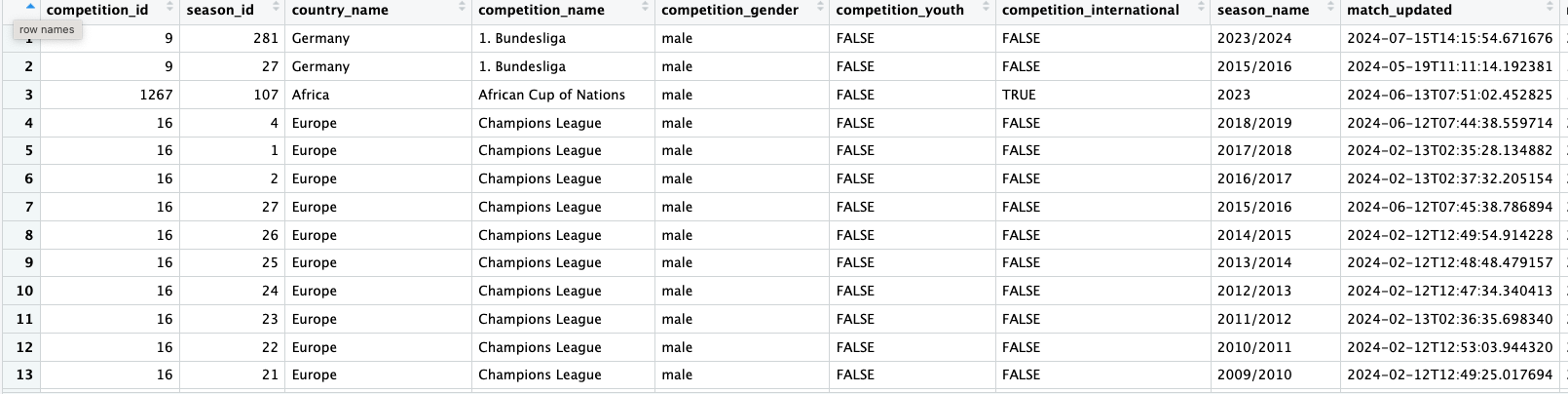
Each competition and season have unique id and we can also see whether it was a men’s or women’s competition. To see which matches from selected competitions have publicly available data, we can pass the corresponding rows of this table to the function StatsBombR::FreeMatches(). For instance, here are the first few rows and some selected columns from the matches from EURO 2022. StatsBomb graciously provided data for all the matches in the tournament. Here is a table of matches from the 2022 EURO Competition; StatsBomb graciously provided data for all matches from the tournament, which can be obtained using the code below.
StatsBombR::FreeCompetitions() |>
  dplyr::filter(competition_id == 53 & season_id == 106) |>
  StatsBombR::FreeMatches() |>
  dplyr::select(match_id, home_team.home_team_name, away_team.away_team_name, home_score, away_score)
[1] "Whilst we are keen to share data and facilitate research, we also urge you to be responsible with the data. Please credit StatsBomb as your data source when using the data and visit https://statsbomb.com/media-pack/ to obtain our logos for public use."
[1] "Whilst we are keen to share data and facilitate research, we also urge you to be responsible with the data. Please credit StatsBomb as your data source when using the data and visit https://statsbomb.com/media-pack/ to obtain our logos for public use."# A tibble: 31 × 5
match_id home_team.home_team_n…¹ away_team.away_team_…² home_score away_score
<int> <chr> <chr> <int> <int>
1 3835331 Sweden Women's Switzerland Women's 2 1
2 3835324 Netherlands Women's Sweden Women's 1 1
3 3844384 England Women's Spain Women's 2 1
4 3847567 England Women's Germany Women's 2 1
5 3845506 England Women's Sweden Women's 4 0
6 3835335 Northern Ireland England Women's 0 5
7 3835323 Portugal Women's Switzerland Women's 2 2
8 3835325 France Women's Italy Women's 5 1
9 3835320 Norway Women's Northern Ireland 4 1
10 3845507 Germany Women's France Women's 2 1
# ℹ 21 more rows
# ℹ abbreviated names: ¹home_team.home_team_name, ²away_team.away_team_nameTo access the raw event-level data from a subset of matches, we need to pass the table above to the function StatsBombR::free_allevents(). StatsBomb also recommends running some basic pre-processing, all of which is nicely packaged together in the functions StatsBombR::allclean() and StatsBombR::get.opposingteam().
As an example, the code chunk below pulls out publicly available event data for every women’s international match.
wi_events <-
StatsBombR::FreeCompetitions() |>
dplyr::filter(competition_gender == "female" & competition_international) |>
StatsBombR::FreeMatches() |>
StatsBombR::free_allevents() |>
StatsBombR::allclean() |>
StatsBombR::get.opposingteam()- 1
- Get table of all available competitions
- 2
- Find all women’s international competition
- 3
- Get table of matches
- 4
- Get all events
- 5
-
allclean()andget.opposingteam()run several pre-processing scripts that StatsBomb recommends.
Developing Complex Pipelines
It is not easy to codepipelines like the above in a single attempt. In fact, I had to build the code line-by-line. For instance, I initially ran just the first line and manually inspected the table of free competitions (using View()) to figure out which variables I needed to filter() on in the second line. It is very helpful to develop pipelines incrementally and to check intermediate results before putting everything together in one block of code.
Estimating Expected Goals
Suppose we observe a dataset consisting of \(n\) shots. For each shot \(i = 1, \ldots, n,\) let \(Y_{i}\) be a binary indicator of whether the shot resulted in a goal (\(Y_{i} = 1\)) or not (\(Y_{i} = 0\)). From the high-resolution tracking data, we can extract a potentially huge number of features about the shot at the moment of it was taken. Possible features include, but are certainly not limited to, the player taking the shot, the body part and side of the body used, the positions of the defenders and goal keepers, and contextual information like the score. Mathematically, we can collect all these features into a (potentially large) vector \(\boldsymbol{\mathbf{X}}_{i}.\)
Expected Goals (XG) models work by (i) positing an infinite super-population of shots represented by pairs \((\boldsymbol{\mathbf{X}}, Y)\) of feature vector \(\boldsymbol{\mathbf{X}}\) and binary outcome \(Y\); and (ii) assuming that the shots in our dataset constitute a random sample \((\boldsymbol{\mathbf{X}}_{1}, Y_{1}), \ldots, (\boldsymbol{\mathbf{X}}_{n}, Y_{n})\) from that population.
Because the shot outcome \(Y\) is binary, \(\textrm{XG}(\boldsymbol{\mathbf{x}})\) is the proportion of goals scored within the sub-population of shots defined by the feature combinations \(\boldsymbol{\mathbf{x}}.\) In other words, it is the conditional probability of a goal given the shot features \(\boldsymbol{\mathbf{x}}.\) On this view, \(\textrm{XG}(\boldsymbol{\mathbf{x}})\) provides a quantitative answer to our motivating question “If we were to replay a particular shot over and over again, what fraction of the time does it result in a goal?”
The StatsBomb variable shot.body_part.name records the body part with which each shot was taken. Within our dataset of women’s international matches, we can see the breakdown of these body parts.
table(wi_events$shot.body_part.name)
      Head  Left Foot      Other Right Foot
       920       1280         27       2560
For this analysis, we will focus on fitting XG models using data from shots taken with a player’s feet or head.
wi_shots <-
  wi_events |>
  dplyr::filter(type.name == "Shot" & shot.body_part.name != "Other") |>
  dplyr::mutate(Y = ifelse(shot.outcome.name == "Goal", 1, 0))
Later, it will be useful for us to focus only on the shots from EURO2022, so we will also create a table euro2022_shots of all shots from that competition using similar code.
Code
euro2022_shots <-
  StatsBombR::FreeCompetitions() |>
  dplyr::filter(competition_id == 53 & season_id == 106) |>
  StatsBombR::FreeMatches() |>
  StatsBombR::free_allevents() |>
  StatsBombR::allclean() |>
  StatsBombR::get.opposingteam() |>
  dplyr::filter(type.name == "Shot" & shot.body_part.name != "Other") |>
  dplyr::mutate(Y = ifelse(shot.outcome.name == "Goal", 1, 0))
Now suppose we only include the body part in \(\boldsymbol{\mathbf{X}}\). If we had full access to the infinite super-population of women’s international shots, then we could compute \[\textrm{XG}(\text{right-footed shot}) = \mathbb{P}(\text{goal} \vert \text{right-footed shot})\] by (i) forming a sub-group containing only those right-footed shots and then (ii) calculating the proportion of goals scored within that sub-group. We could similarly compute \(\textrm{XG}(\text{left-footed shot})\) and \(\textrm{XG}(\text{header})\) by calculating the proportion of goals scored within the sub-groups containing, respectively, only left-footed shots and only headers.
Of course, we don’t have access to the infinite super-population of shots. However, on the assumption that our observed data constitute a sample from that super-population, we can estimate \(\textrm{XG}\) by mimicking the idealized calculations described above:
- Break the dataset of all observed shots in women’s international matches into several groups based on the body part
- Within these two groups, compute the proportion of goals
To keep things simple, we dropped the 23 shots that were taken with a body part other than the feet or the head.
xg_model1 <-
  wi_shots |>
  dplyr::group_by(shot.body_part.name) |>
  dplyr::summarise(XG1 = mean(Y), n = dplyr::n())
xg_model1
# A tibble: 3 × 3
shot.body_part.name XG1 n
<chr> <dbl> <int>
1 Head 0.112 920
2 Left Foot 0.114 1280
3 Right Foot 0.111 2560
Generalization
A key assumption of all XG models is that the observed data is a random sample drawn from the super-population. The only women’s internationals matches for which StatsBomb data were from the 2019 and 2023 World Cup and the 2022 and 2025 EURO tournaments. These matches are arguably not highly representative of all women’s international matches, meaning that we should exercise some caution when using models fitted to these data to analyze matches from other competitions (e.g., an international friendly or a match in a domestic league).
We can now create a table of just Beth Mead’s shots from EURO 2022 and add a column with the XG for each shot. To do this, we first filter our table wi_shots using the player name (note, StatsBomb uses her full name!). Then, for every left-footed shot Mead attempted, we want to copy over the corresponding value from the table xg_model1, which in this case is 0.114. Similarly, we want to copy over the corresponding values for right-footed shots and headers from xg_model1 into our table for Mead’s shots. We can do this using an left join. In the code below, we actually create a temporary version of xg_model1 that drops the column recording the overall counts of the body part used for the shots in wi_shots. This way, when we perform the join, we don’t create a new column with these counts.
mead_shots <-
euro2022_shots |>
dplyr::filter(player.name == "Bethany Mead") |>
dplyr::left_join(y = xg_model1 |> dplyr::select(shot.body_part.name, XG1),
by = c("shot.body_part.name"))- 1
-
No need to include
nwhen joining the tables
We can now look at the what our model says about the three goals from above. The first, against Austria in the 15th minute; the second, against Norway in the 37th minute, and the third against Sweden in the 33rd minute. These turn out to be in rows 1, 4, and 14 of the table mead_shots
mead_shots |>
  dplyr::select(OpposingTeam, minute, shot.body_part.name, Y, XG1) |>
  dplyr::slice(c(1, 4, 14))
# A tibble: 3 × 5
OpposingTeam minute shot.body_part.name Y XG1
<chr> <int> <chr> <dbl> <dbl>
1 Austria Women's 15 Right Foot 1 0.111
2 Norway Women's 37 Left Foot 1 0.114
3 Sweden Women's 33 Right Foot 1 0.111According to our first model, the “impressiveness” of these goals is pretty similar: our model put the respective chances of each shot resulting in a goal at about 11%. But, watching the videos a bit more closely, this conclusion is not especially satisfying: Mead scored the first goal in a one-on-one situation but had to shoot through several defenders on the second and third goal. The discrepancy between our qualitative comparisons and our quantitative modeling results stems from the fact that we only conditioned on the body part and did not account for the other ways that the shots are different. In other words, our initial XG model is much too coarse to quantify the differences between the three chances that we believe are important.
Conditioning On Additional Features
For a more refined comparison, we need an XG model that conditions on more features, including ones that differ between the two shots. To this end, notice that Mead uses a different technique on the three shots: she lobs the ball into the net on the first goal; shoots the ball from the ground on the second goal; and scores the third goal off of a half-volley, striking the ball as it bounces up off the ground. The StatsBomb variable shot.technique.name records the technique of each shot type
table(wi_shots$shot.technique.name)
     Backheel Diving Header   Half Volley           Lob        Normal
           35            10           648            28          3720
Overhead Kick        Volley
           17           302
By conditioning on both body part and technique, we can begin to build a more refined XG model. The code to do this is almost identical to the code used in our first model. The only difference is that we now group by two variables shot.body_part.name and shot.technique_name. Because we are grouping by two variables, specify the argument .groups="drop" argument when calling summarize; this prevents a (mostly innocuous) warning message2. We additionally append our new XG estimates to the table containing all of Mead’s shots.
xg_model2 <-
  wi_shots |>
  dplyr::group_by(shot.body_part.name, shot.technique.name) |>
  dplyr::summarize(XG2 = mean(Y), n = dplyr::n(), .groups = "drop")

mead_shots <-
  mead_shots |>
  dplyr::inner_join(
    y = xg_model2 |> dplyr::select(-n),
    by = c("shot.body_part.name", "shot.technique.name"))

mead_shots |>
  dplyr::select(OpposingTeam, minute, shot.body_part.name, shot.technique.name, Y, XG2) |>
  dplyr::slice(c(1, 4, 14))
# A tibble: 3 × 6
OpposingTeam minute shot.body_part.name shot.technique.name Y XG2
<chr> <int> <chr> <chr> <dbl> <dbl>
1 Austria Women's 15 Right Foot Lob 1 0.208
2 Norway Women's 37 Left Foot Normal 1 0.121
3 Sweden Women's 33 Right Foot Half Volley 1 0.0892More Sophisticated XG Models
According to our new XG model, the right-footed lob against Austria has a much higher XG than the other shots against Norway and Sweden, which seems much more reasonable than our previous model. But are we fully satisfied with this model?
One could credibly argue that even though our model returns somewhat more sensible XG estimates, it is still too coarse for to meaningfully compare the shots above. After all, because it does not condition on distance, our model would return exactly the same XG for right-footed volleys taken one meter and 15 meters away from the goal. Similarly, we could try to account for the number of defenders between the shot and the goal and the position of the keeper.
If we had access to the infinite super-population of shots, conditioning on even more features is conceptually straightforward: we look at the corresponding sub-group of the super-population defined by a particular combination of features and compute the average \(Y.\) Unfortunately, with finite data, trying to “bin-and-average” using lots of features can lead to erratic estimates. For instance, here are the five largest and five smallest XG estimates based on body-part and shot technique.
xg_model2 |>
  dplyr::arrange(dplyr::desc(XG2)) |>
  dplyr::filter(dplyr::row_number() %in% c(1:5, (dplyr::n()-4):dplyr::n()))
# A tibble: 10 × 4
shot.body_part.name shot.technique.name XG2 n
<chr> <chr> <dbl> <int>
1 Right Foot Lob 0.208 24
2 Left Foot Volley 0.163 98
3 Left Foot Normal 0.121 947
4 Right Foot Normal 0.121 1863
5 Head Normal 0.113 910
6 Right Foot Volley 0.0637 204
7 Head Diving Header 0 10
8 Left Foot Backheel 0 6
9 Left Foot Lob 0 4
10 Left Foot Overhead Kick 0 3Because none of the 3 left-footed lobs in our dataset led to goals, our model estimates \(\textrm{XG}(\text{left-footed lob})\) as 0. Similarly, the rather large \(\textrm{XG}(\text{right-footed lob})\) of 33% is based on only 12 shots. Attempting to condition on even more variables would result in estimates based on even smaller sample sizes3.
So, it would appear that we’re stuck between a rock and a hard place. On the one hand, our XG model with two features is still too coarse to quantify important differences between the motivating shots. But, on the other hand, binning and averaging with even more features carries the risk of producing highly erratic, extreme, and somewhat nonsensical estimates4.
Statistical models offer a principled approach to overcome these issues. We will explore several such models in Lecture 3. But for now, we will rely on a model developed by StatsBomb that accounts for a large number of features based on player locations (in two dimensions), the ball location (in three dimension), and other factors like the body part, shot technique, and the actions leading up to the shot (e.g., whether shot was taken off dribble or first touch). You can read more about their model here. Luckily for us, they include XG estimates for each shot in the public data, under the column shot.statsbomb_xg.
For instance, here are the XG estimates from StatsBomb’s model for all of Beth Mead’s goals
mead_shots |>
  dplyr::filter(Y == 1) |>
  dplyr::select(OpposingTeam, minute, shot.body_part.name,
                shot.technique.name, Y, shot.statsbomb_xg)
# A tibble: 6 × 6
OpposingTeam minute shot.body_part.name shot.technique.name Y
<chr> <int> <chr> <chr> <dbl>
1 Austria Women's 15 Right Foot Lob 1
2 Norway Women's 33 Head Normal 1
3 Norway Women's 37 Left Foot Normal 1
4 Norway Women's 80 Left Foot Volley 1
5 Northern Ireland 43 Left Foot Normal 1
6 Sweden Women's 33 Right Foot Half Volley 1
# ℹ 1 more variable: shot.statsbomb_xg <dbl>Recall that XG quantifies a certain hypothetical long-term frequency of scoring a goal: if the shot was replayed under exactly the conditions quantified by the feature vector \(\boldsymbol{\mathbf{x}}\), \(\textrm{XG}(\boldsymbol{\mathbf{x}})\) is the proportion of times a goal is scored. So, according to StatsBomb’s proprietary model, if Mead repeatedly attempted the three shots introduced in Section 1.1, we should expect them to result in goals 36%, 44%, and 9% of the time. In other words, according to StatsBomb’s model, Meads goal against Sweden is much more impressive than her goals against Austria and Norway. One could argue, further, that this goal was somewhat lucky.
We can also look at the XG’s of the shots Mead took that didn’t result in goals.
mead_shots |>
  dplyr::filter(Y == 0) |>
  dplyr::select(OpposingTeam, minute, shot.body_part.name,
                shot.technique.name, Y, shot.statsbomb_xg)
# A tibble: 9 × 6
OpposingTeam minute shot.body_part.name shot.technique.name Y
<chr> <int> <chr> <chr> <dbl>
1 Norway Women's 29 Right Foot Normal 0
2 Norway Women's 52 Right Foot Volley 0
3 Northern Ireland 5 Head Normal 0
4 Northern Ireland 15 Right Foot Half Volley 0
5 Northern Ireland 56 Right Foot Normal 0
6 Northern Ireland 83 Right Foot Normal 0
7 Sweden Women's 4 Head Normal 0
8 Sweden Women's 19 Left Foot Normal 0
9 Sweden Women's 46 Left Foot Normal 0
# ℹ 1 more variable: shot.statsbomb_xg <dbl>We see that most of Mead’s misses were on shots with very low XG values, indicating that none of these misses were especially unlucky.
Goals Over Expected
By summing the differences \(Y_{i} - \textrm{XG}_{i}\) across all of her shots, we can quantify the degree to which Mead under- or over-performed the model expectations.
sum(mead_shots$Y - mead_shots$shot.statsbomb_xg)[1] 2.896323We conclude that during EURO 2022, Beth Mead scored 2.9 more goals than what StatsBomb’s XG model expected based on the contexts in which she attempted shots. We can repeat this calculation — summing over the difference between shot outcome \(Y\) and \(\textrm{XG}\) — for all players in EURO 2022 to find the players that most over-performed and most under-performed the model expectations.
goe <-
  euro2022_shots |>
  dplyr::mutate(diff = Y - shot.statsbomb_xg) |>
  dplyr::group_by(player.name) |>
  dplyr::summarise(GOE = sum(diff),n = dplyr::n()) |>
  dplyr::arrange(dplyr::desc(GOE))
goe
# A tibble: 200 × 3
player.name GOE n
<chr> <dbl> <int>
1 Alexandra Popp 3.34 16
2 Bethany Mead 2.90 15
3 Alessia Russo 1.79 12
4 Francesca Kirby 1.79 5
5 Lina Magull 1.70 14
6 Ingrid Filippa Angeldal 1.37 10
7 Romée Leuchter 1.19 2
8 Hanna Ulrika Bennison 0.952 1
9 Nicole Anyomi 0.896 1
10 Julie Blakstad 0.879 1
# ℹ 190 more rowsIt turns out that Alexandra Popp, the German captain, outperformed StatsBomb’s XG model expectations by an even wider margin than Beth Mead. Like Mead, Popp scored 6 goals during the tournament off a similar number of shots (16 for Popp and 15 for Mead). Interestingly, Mead won the Golden Boot because she had one more assist…
Exercises
- For each team in EURO 2022, sum the \(\textrm{XG}_{i}\) values and sum the residuals \(Y_{i} - \textrm{XG}_{i}.\) Which teams most over- or under-performed expectations? What relationship, if any, do you observe between teams’ cumulative XG and their performance relative to the StatsBomb XG model’s expectations?
- Hudl recently released data from EURO 2025. Repeat the analysis from Section 6 to identify the players with the most extreme goals over expected values from the tournament.
- Repeat Exercise 2.1 using data from EURO 2025
- Hudl also release several full seasons worth of data from professional leagues. Pick one such season and explore the relationships between (i) the cumulative XG the team generates on offense; (ii) the cumulative XG the team gives up on defense; and (iii) the win-loss record across the season.
References
Lindley, Dennis. 1985. Making Decisions. Wiley.
Footnotes
And props to Hudl for continuing to make this data available!↩︎
See this StackOverflow post and the documentation for
summarisefor details.↩︎Try to convince yourself why this is the case!↩︎
Indeed, it seems absurd to claim that, at least in women’s international soccer, players will never score off left-footed lobs! As the Statistician Dennis Lindley put it, we must “never believe in anything absolutely” and we should “leave a little probability for the moon being made of green cheese; it can be as small as 1 in a million, but have it there since otherwise an army of astronauts returning with samples of the said cheese will leave you unmoved” (Lindley 1985, sec. 6.7, available here). Lindley termed this principle “Cromwell’s Rule”, a reference to Oliver Cromwell’s quote “I beseech you, in the bowels of Christ, think it possible that you may be mistaken” from his letter to the Church of Scotland.↩︎