pbp2024 <-
  nflfastR::load_pbp(season = 2024) |>
  dplyr::filter(season_type == "REG")
roster2024 <-
  nflfastR::fast_scraper_roster(seasons = 2024) |>
dplyr::filter(!is.na(gsis_id))Lecture 10: NFl WAR
Overview
In Lecture 9, we looked at two touchdowns from the 2024-25 NFL season:
- A 86-yard touchdown by Ladd McConckey on a pass from Justin Herbert (video link)
- A 64-yard touchdown by Kavontae Turpin on a pass from Cooper Rush (video link)
The McConckey touchdown was thrown on a 3rd and 26 from the Charger’s 14 yard line. From that position, teams are expected to score about -1.54 points; that is, starting from that positions, teams, on average, give up points rather than score them. Over the course of the play, the Chargers offense generated around 8.54 points of EP. The Turpin touchdown, on the other hand, was thrown on a 3rd and 10 from the Cowboys’ 36 yard line, a position from which teams score about 0.77 on average. The Cowboys offense generated about 6.23 points of EPA during that play. How much of the created EPA on these plays should be credited to the quarterbacks and how much should be credited to the receivers? Which players
In this lecture, we will use multilevel modeling to answer these questions. We separately model EPA on passing and running plays. For passing plays, we will decompose the EPA into two parts, the expected points gained while the pass is in the air and the expected points gained on the ground after the catch (if the pass was caught). Each of our multilevel models will include random intercepts for players nested by their position (e.g., passer and receiver in the passing EPA models) and will also adjust for several important fixed effects. From these models, we will determine how many more expected points per play each player adds relative to the league average. Finally, like we did in Lecture 8, we will translate these expected points added to the win scale and conclude with a version of wins above replacement for offensive players in football. Our development closely follows the nflWAR model introduced by Yurko, Ventura, and Horowitz (2019) but makes some simplifications.
Data Preparation
We will restrict our analysis to plays from the 2024-25 regular season and exclude all post-season/play-off games. Later, in Section 5.1, we will define replacement-level players on a position-by-position basis. So that we can look up player positions, we will re-load the roster information using nflfastR::fast_scraper_roster().
Passing Plays Data
We will extract information about all passing plays from pbp2024 into a data table called pass2024.
pass2024 <-
pbp2024 |>
dplyr::filter(
play_type == "pass" &
!is.na(posteam) &
!grepl("TWO-POINT CONVERSION ATTEMPT", desc) &
!grepl("sack", desc) ) |>
dplyr::filter(passer_player_id != receiver_player_id) |>
dplyr::select(
passer_player_id,
receiver_player_id,
posteam, defteam,
air_yards, shotgun,
qb_hit, no_huddle,
posteam_type,
pass_location,
yards_after_catch,
epa, air_epa, yac_epa, complete_pass, desc) |>
dplyr::mutate(gsis_id = receiver_player_id) |>
dplyr::left_join(y = roster2024 |> dplyr::select(gsis_id, position), by = "gsis_id") |>
dplyr::rename(receiver_position = position) |>
dplyr::select(-gsis_id)- 1
- Remove pass attempts on two-point conversions
- 2
- nflfastR classifies sacks as passing plays. For the purposes of building a version of WAR for the NFL, we will treat sacks as running plays, similar to Yurko, Ventura, and Horowitz (2019).
- 3
- Remove plays like this where the passer catches their own pass (usually off a deflection).
- 4
- Copy receiver ID into a temporary column, which will be used append receiver position with a join.
- 5
- Append receiver position.
- 6
- Rename the column containing receiver position.
- 7
- Remove the temporary column holding the receiver ID
In addition to the identity of the passer (passer_player_id) and intended receiver (receiver_player_id), the data table contains the following columns: * posteam: the identity of the team in possession of the ball * defteam: the identity of the team on defense * air_yards: the distance traveled by the pass through the air[^airyard] * shotgun: whether the pass was thrown out of the shotgun formation * qb_hit: whether the quarterback was hit while throwing * no_huddle: whether the play was run without a huddle * posteam_type: whether the home team had possession (i.e., was on offense) * pass_location: whether the pass was thrown to the left, right, or center of the field * yards_after_catch: for completions, how many yards did the receiver gain after catching the pass * epa: the expected points added on the play * air_epa and yac_epa: the expected points added through the air and running after the catch (for completed passes) * complete_pass: whether the pass was completed * receiver_position: the position of the actual receiver on completed passes and the intended receiver on incomplete passes
For every passing play, nflfastR computes two different EPA values. The first, air_epa is the expected points added through the air and yac_epa is the expected points added after the catch. For completed passes, computing air_epa and yac_epa is relatively straightforward: as soon as the pass is caught, imagine stopping the play and computing the expected points based on the resulting game state. Then, the difference between this intermediate EP and the starting EP of the original play is air_epa and the difference between the final EP and this intermediate EP is yac_epa. Computing air_epa and yac_epa for incomplete passes is trickier and involves computing the difference in expected points between the final state, initial state, and an intermediate state that would result had the pass been caught.
Rushing Plays Data
Success in the run game depends not only on the skill of the individual runner to run through the space created by his teammates and evade defenders but also on the ability of his teammates (usually linemen) to create space near the line and to make blocks down the field. Unfortunately, publicly available NFL play-by-play does not record the identities of all 22 players on the field nor does it include information about play (i.e., whether the play involved a pulling guard). It does, however, contain two variables, run_location, and run_gap that provide some context about the play.
We start by building a data table containing all rushing plays. As noted above, we will treat sacks as rushing plays.
rush2024 <-
pbp2024 |>
dplyr::filter(
!grepl("TWO-POINT CONVERSION ATTEMPT", desc)) |>
dplyr::filter(
!grepl("No play", desc, ignore.case = TRUE)) |>
dplyr::filter(
play_type == "run" |
grepl("sack", desc, ignore.case = TRUE)) |>
dplyr::select(
game_id, play_id,
posteam, defteam,
passer_player_id,
rusher_player_id,
posteam_type,
shotgun, no_huddle,
run_location, run_gap,
epa, desc) - 1
- Remove the plays that are whistled dead or involve penalties like roughing the passer or are otherwise classified as “No Play”
- 2
- On sacks, the quarterback is sometimes not classified as a runner but as passer
The data table rush2024 contains several of the same variables pass2024 including the identities of the offensive and defensive teams, the EPA, and the indicators shotgun, no_huddle, and posteam_type. It also includes the ID for the runner and their listed position and two variables, run_location and run_gap, that contain some contextual information about the run. Unfortunately, there are a lot of missing values of rusher_player_id, all of which correspond to sacks.
sum(is.na(rush2024$rusher_player_id))[1] 1327sum(grepl("sack", rush2024$desc, ignore.case = TRUE) & is.na(rush2024$rusher_player_id))[1] 1327Handling Sacks
nflfastR treats sacks as passing plays and not running plays. However, because the ball is not thrown during a sack, there is no well-defined air_epa or yac_epa. We instead follow the example of Yurko, Ventura, and Horowitz (2019) and treat sacks as running plays. Unfortunately, for the vast majority of sacks, the rusher_player_id variable is not available.
sacks <-
  rush2024 |>
  dplyr::filter(grepl("sack", desc, ignore.case = TRUE))
mean(is.na(sacks$rusher_player_id))
[1] 0.999247Instead, the id of the player who was sacked — whom we wish to treat as the rusher in our models — is saved as passer_player_id. We first verify that all sacks with a missing rusher_player_id do not also have a missing passer_player_id
sum(is.na(sacks$rusher_player_id))
sum(!is.na(sacks$passer_player_id) & is.na(sacks$rusher_player_id))- 1
-
Number of sacks for which we are missing the
rusher_player_id - 2
-
Number of sacks for which are missing the
rusher_player_idbut are not missing thepasser_player_id
[1] 1327
[1] 1327
The following code overwrites the missing rusher_player_id values on sacks and then appends the rusher’s position.
rush2024 <-
  rush2024 |>
  dplyr::mutate(
    rusher_player_id =
      dplyr::case_when(
        is.na(rusher_player_id) & grepl("sack", desc, ignore.case = TRUE) ~ passer_player_id,
        .default = rusher_player_id)) |>
  dplyr::mutate(gsis_id = rusher_player_id) |>
  dplyr::left_join(y = roster2024 |> dplyr::select(gsis_id, position), by = "gsis_id") |>
  dplyr::rename(rusher_position = position) |>
  dplyr::select(-gsis_id)
Run Context
The data table rush2024 contains two variables that describe the run play. The first, run_location, records whether the run was towards the left, right or middle of the offensive line. To describe run_gap, we need to introduce a little bit of additional notation. Every offensive play in American football begins with 5 offensive players (the “linemen”) on the line of scrimmage. The center is responsible for snapping the ball to the quarterback — thereby starting the play — and is positioned in the middle of the line. Next to the center are the two guards and next to the guards are the two tackles. The spaces between the linemen are known as “gaps” and are conventionally labelled with letters: “A” gap between the center and guard; “B” gap between guard and tackle, and “C” gap outside the tackle. Sometimes, but not always, a tight end lines up next to one or both of the tackles. When that happens, the space between the tackle and end is labelled “C” gap and the space outside the tight end is known as “D” gap.
Although the naming convention is very prevalent within football (i.e, amongst coaches and players), the NFL play-by-play data does not use this convention. Instead, the variable run_gap takes the value guard for runs through the “B” gap, tackle for runs through the “C” gap, and end for runs through the “D” gap. For runs through the “B”, “C”, or “D” gap, the variable run_location takes on the value “left” or “right”, to indicate which side of the line But for runs through the “A” gap, run_gap is NA and run_location is equal to “middle”.
table(rush2024[,c("run_gap", "run_location")], useNA = 'always') run_location
run_gap left middle right <NA>
end 1958 0 1805 0
guard 1822 0 1739 0
tackle 1645 0 1628 0
<NA> 0 3565 0 1447We will combine these two variables into a composite variable run_context. For runs where both run_gap and run_location are not NA, we will concatenate the three variables (e.g., "left end" or "right tackle"). For runs through the “A” gap (when run_location == "middle" and run_gap is NA), we will set the contextual variable to be "middle". It turns out that the remaining 1447 running plays with missing run_location and run_gap involve a sack or fumble (and sometimes both!)
tmp <-
rush2024 |>
dplyr::filter(is.na(run_gap) & is.na(run_location))
all(
grepl("sack", tmp$desc, ignore.case = TRUE) | #<3
grepl("fumble", tmp$desc, ignore.case = TRUE) )- 1
-
Pull out all the plays missing both
run_gapandrun_location. - 2
-
allreturnsTRUEif all elements in a logical vector are true - 3
- Check whether the strings “sack” or “fumble” appears in the play description.
[1] TRUEFor these plays, we will set run_context == "other". We further combine run_context with the identity of the offensive team (i.e., posteam) to create what Yurko, Ventura, and Horowitz (2019) describe as a “proxy for the offensive linemen or blockers involved in a rushing attempt.”
rush2024 <-
  rush2024 |>
  dplyr::mutate(
    run_context = dplyr::case_when(
      run_location == "middle" ~ paste(posteam, "middle", sep = "_"),
      is.na(run_location) & is.na(run_gap) ~ paste(posteam, "other", sep = "_"),
      .default = paste(posteam, run_gap, run_location, sep = "_")))
Accounting for Team Strengths
Recall one of the main drawbacks of plus/minus was its inability to account for the quality of the player’s teammates. When trying to construct a version of WAR for offensive players in the NFL, we need to make sure that we do not overly reward players who happen to play for good teams or overly penalize players who play on bad offenses. In our multilevel models, we will quantify each offense’ running and passing strength using the average EPA on rushing and passing plays.
pass_strength <-
  pass2024 |>
  dplyr::group_by(posteam) |>
  dplyr::summarise(pass_strength = mean(epa,na.rm = TRUE))
rush_strength <-
  rush2024 |>
  dplyr::group_by(posteam) |>
  dplyr::summarise(rush_strength = mean(epa, na.rm = TRUE))


pass2024 <-
  pass2024 |>
  dplyr::inner_join(pass_strength, by = "posteam") |>
  dplyr::inner_join(rush_strength, by = "posteam")

rush2024 <-
  rush2024 |>
  dplyr::inner_join(pass_strength, by = "posteam") |>
  dplyr::inner_join(rush_strength, by = "posteam")
Passing Models
Constructing Composite Outcomes
We’re now ready to determine how much individual players contribute to their team’s overall EPA on passing plays. While it is tempting to fit separate multilevel models to predict the values in the air_epa and yac_epa, we need to be a bit more careful in how we deal with incomplete passes. Specifically, on an incomplete pass, there is necessarily no run after the catch and any change in EP is driven entirely by what happens while the ball is in the air. To account for this, we will define two composite outcomes that are based on air_epa, yac_epa, and epa.
Formally, say that there are \(n\) passing plays and for passing play \(i,\) let \(\Delta_{i}\) be the observed EPA on the play. Let \(\delta_{i,\textrm{air}}\) and \(\delta_{i,\textrm{yac}}\) be the values of air_epa and yac_epa provided by nflfastR. We will decompose \(\Delta_{i} = \Delta_{i,\textrm{air}} + \Delta_{i,\textrm{yac}}\) where \[
\Delta_{i, \textrm{air}} =
\begin{cases}
\delta_{i, \textrm{air}} & \textrm{if the pass is caught} \\
\Delta_{i} & \textrm{if the pass is incomplete,}
\end{cases}
\] and \[
\Delta_{i, \textrm{yac}} =
\begin{cases}
\delta_{i, \textrm{yac}} & \textrm{if the pass is caught} \\
0 & \textrm{if the pass is incomplete.}
\end{cases}
\] The following code creates columns for these composite outcomes and also converts categorical predictors like defensive team and receiver position into factor variables.
pass2024 <-
  pass2024 |>
  dplyr::mutate(
    Delta_air = ifelse(complete_pass == 1, air_epa, epa),
    Delta_yac = ifelse(complete_pass == 1, yac_epa, 0),
    passer_player_id = factor(passer_player_id),
    receiver_player_id = factor(receiver_player_id),
    posteam = factor(posteam),
    defteam = factor(defteam),
    pass_location = factor(pass_location),
    receiver_position = factor(receiver_position))
Modeling \(\Delta_{\textrm{air}}\)
Our first multilevel model, fitted to data from all passing plays, includes separate random intercepts for the passers, receivers, and defenses. It also accounts for the fixed effects of * air_yards: the distance traveled by the pass through the air * shotgun: whether the pass was thrown out of the shotgun formation * qb_hit: whether the quarterback was hit while throwing * no_huddle: whether the play was run without a huddle * posteam_type: whether the home team had possession (i.e., was on offense) * pass_location: whether the pass was thrown to the left, right, or center of the field * receiver_position: the position of the intended receiver * rush_strength: the average EPA per rush attempt for the offense
Before writing down our model, we introduce some more notation. Formally, suppose that there are \(n_{q}\) passers1, \(n_{c}\) receivers2, and \(n_{D}\) defenses. For passing play \(i,\) let \(q[i], c[i],\) and \(d[i]\) denote the identity of the passer, receiver, and defense involved in the play and let \(\boldsymbol{\mathbf{x}}_{i}\) be the vector of fixed effect covariates (i.e., the ones listed above).
We model \[ \begin{align} \Delta_{i, \textrm{air}} &= Q_{q[i]} + C_{c[i]} + D_{d[i]} + \boldsymbol{\mathbf{x}}_{i}^{\top}\boldsymbol{\beta} + \epsilon_{i} \quad \text{for all passes}\ i = 1, \ldots, n \\ Q_{q} &\sim N(\mu_{Q}, \sigma^{2}_{Q}) \quad \textrm{for all passers}\ q = 1, \ldots, n_{Q} \\ C_{c} &\sim N(\mu_{C}, \sigma^{2}_{C}) \quad \textrm{for all pass catchers}\ c = 1, \ldots, n_{C}, \\ D_{d} &\sim N(\mu_{D}, \sigma^{2}_{D}) \quad \textrm{for all defenseive teams}\ d = 1, \ldots n_{D}. \end{align} \]
We can fit this model with lme4::lmer() using similar notation as was used in Lecture 9. Just like in that lecture, we can read off lots of important information and parameter estimates from the model summary. For instance, there is much more variability in the receiver effects than the passer or defense effects.
library(lme4)- 1
- We want random intercepts for the passer, receiver, and defensive team
- 2
- Specify the fixed effects
Loading required package: Matrixair_model <-
lmer(Delta_air ~ 1 + (1|passer_player_id) + (1 | receiver_player_id) + (1 | defteam )
+ air_yards + shotgun + qb_hit + no_huddle + posteam_type + pass_location + receiver_position + rush_strength,
data = pass2024)
summary(air_model)
Correlation matrix not shown by default, as p = 16 > 12.
Use print(x, correlation=TRUE)  or
    vcov(x)        if you need it
Linear mixed model fit by REML ['lmerMod']
Formula: Delta_air ~ 1 + (1 | passer_player_id) + (1 | receiver_player_id) +
(1 | defteam) + air_yards + shotgun + qb_hit + no_huddle +
posteam_type + pass_location + receiver_position + rush_strength
Data: pass2024
REML criterion at convergence: 56640.3
Scaled residuals:
Min 1Q Median 3Q Max
-9.6663 -0.4475 -0.0140 0.4521 4.2381
Random effects:
Groups Name Variance Std.Dev.
receiver_player_id (Intercept) 0.011544 0.10745
passer_player_id (Intercept) 0.002242 0.04735
defteam (Intercept) 0.001354 0.03680
Residual 1.622752 1.27387
Number of obs: 17000, groups:
receiver_player_id, 492; passer_player_id, 99; defteam, 32
Fixed effects:
Estimate Std. Error t value
(Intercept) -2.642055 0.573232 -4.609
air_yards 0.035027 0.001077 32.537
shotgun -0.081497 0.028132 -2.897
qb_hit -0.276667 0.036182 -7.647
no_huddle 0.134666 0.029805 4.518
posteam_typehome -0.008663 0.019728 -0.439
pass_locationmiddle 0.172170 0.026424 6.516
pass_locationright -0.034797 0.022336 -1.558
receiver_positionDL 4.627420 1.401649 3.301
receiver_positionLB 3.750986 1.070748 3.503
receiver_positionOL 2.527147 0.729736 3.463
receiver_positionQB 3.661843 0.934966 3.917
receiver_positionRB 1.922465 0.573394 3.353
receiver_positionTE 2.279044 0.573261 3.976
receiver_positionWR 2.254500 0.573040 3.934
rush_strength 0.307995 0.118268 2.604For each passer \(q,\) \(Q_{q}\) is a latent3 quantity measuring how many expected points passer \(q\) adds through the air, after you account for the fixed effects and also the quality of the intended receiver and the defense. The quantity \(\mu_{Q}\) represents the global average of these latent quantities. Similarly, \(C_{c}\) is the latent measurement of how many expected points receiver \(c\) adds while the pass is in the air4 after accounting for the fixed effects and the quality of the passer and of the opposing defense. And \(D_{d}\) is the latent measurement of how many expected points are added for the offensive team by defensive team \(d\) while the pass is in the air. Since EPA is signed so that positive values are considered good for the offense, large negative values of \(D_{d}\) are treated as good for the defense. In our model, the random intercepts \(Q_{q}, C_{c},\) and \(D_{d}\) are all modeled as noisy deviations away from league-wide averages \(\mu_{Q}, \mu_{C},\) and \(\mu_{D}.\)
Unfortunately, we cannot estimate \(\mu_{Q}, \mu_{C},\) and \(\mu_{D}\) because these parameters are not identified. Without going into too many technical details5, there are infinitely many settings of the values of these three parameters that yield exactly the same fit to the data. Because we cannot estimate \(\mu_{Q}, \mu_{C},\) and \(\mu_{D},\) we are unable to obtain estimates for the random intercepts \(Q_{q}, C_{c},\) and \(D_{d}\) like we did in Lecture 9. We are, however, able to estimate the deviations \(Q_{q} - \mu_{Q},\) \(C_{c} - \mu_{C},\) and \(D_{d} - \mu_{D}.\) For each passer \(q\), the quantity \(Q_{q} - \mu_{Q}\) measures many more expected points per play passer \(q\) adds through the air than the league average. Following Yurko, Ventura, and Horowitz (2019), we will refer to this number as passer \(q\)’s individual points added over average or \(\textrm{IPA}^{(Q)}_{\textrm{air},q}\)6. We can similarly define \(\textrm{IPA}^{(C)}_{\textrm{air}, c}\) for receivers. For each defense \(d,\) let \(D_{d} - \mu_{D}\) is the number of points per passing play over league average given up by the defensive team while the bar is in the air. We will denote this quantity by \(\textrm{TPA}^{(D)}_{\textrm{air},d},\) with negative \(\textrm{TPA}\) values corresponding to better defenses.
We can extract the IPA and TPA values using the function ranef().
tmp_air <- ranef(air_model)
air_passer_effects <-
data.frame(
gsis_id = rownames(tmp_air[["passer_player_id"]]),
ipa_air_pass = tmp_air[["passer_player_id"]][,1])
air_receiver_effects <-
data.frame(
gsis_id = rownames(tmp_air[["receiver_player_id"]]),
ipa_air_rec = tmp_air[["receiver_player_id"]][,1])
air_defense_effects <-
data.frame(
Team = rownames(tmp_air[["defteam"]]),
tpa_air_def = tmp_air[["defteam"]][,1])- 1
- Extract the passer, receiver, and defensive random intercepts in a large list
- 2
-
Because we will eventually append player names by
inner_join()’ing withroster2024, we’ll record the passer IDs in a column calledgsis_id.
Taking a quick look at the top-5 (resp. bottom-5) IPA passer values, we see a number of highly regarded (resp. heavily criticized) quarterbacks.
air_passer_effects |>
  dplyr::inner_join(y = roster2024 |> dplyr::select(gsis_id, full_name), by = "gsis_id") |>
  dplyr::select(full_name, ipa_air_pass) |>
  dplyr::arrange(dplyr::desc(ipa_air_pass)) |>
  dplyr::slice(c(1:5, (dplyr::n()-4):dplyr::n()))
full_name ipa_air_pass
1 Joe Burrow 0.06736333
2 Sam Darnold 0.04033663
3 Lamar Jackson 0.03292716
4 Tua Tagovailoa 0.03281935
5 Brock Purdy 0.03000549
6 Drew Lock -0.02737783
7 Bo Nix -0.02808707
8 Dorian Thompson-Robinson -0.03832239
9 Spencer Rattler -0.05005097
10 Anthony Richardson -0.07074920Modeling \(\Delta_{\textrm{yac}}\)
By fitting a similar multilevel model to predict the \(\Delta_{i, \textrm{yac}}\)’s, we can estimate how much each passer, receiver, and defense contributes to EPA during the part of a passing play following a catch. Because these contributions can, by definition, only be made following a completed pass, we fit this model using only the data from completed pass7.
completions <-
  pass2024 |>
  dplyr::filter(complete_pass==1)

yac_model <-
  lmer(Delta_yac ~ 1 + (1|passer_player_id) + (1 | receiver_player_id) + (1 | defteam )
       + air_yards + shotgun + qb_hit + no_huddle + posteam_type + pass_location + receiver_position + rush_strength,
       data = completions)
boundary (singular) fit: see help('isSingular')While fitting the model, lmer printed a message saying that the fit was singular. The manual page for isSingular, which the message instructs us to visit, contains lots of information about singular models. Briefly, when fitting complicated multilevel models with lots of random effects, it can sometimes be the case that some of the “between” group variances are estimated to be exactly zero. Quoting from the manual
While singular models are statistically well-defined … there are real concerns that (1) singular fits correspond to overfitted models that may have poor power; (2) chances of numerical problems or mis-convergence are higher for singular models … ; (3) standard inferential procedures such as Wald statistics and likelihood ratio tests may be inappropriate.
Taking a look at the model summary, we see that the passer-to-passer variation has been set to zero.
summary(yac_model)Linear mixed model fit by REML ['lmerMod']
Formula: Delta_yac ~ 1 + (1 | passer_player_id) + (1 | receiver_player_id) +
(1 | defteam) + air_yards + shotgun + qb_hit + no_huddle +
posteam_type + pass_location + receiver_position + rush_strength
Data: completions
REML criterion at convergence: 32367.4
Scaled residuals:
Min 1Q Median 3Q Max
-8.9533 -0.5437 -0.2533 0.2882 7.4637
Random effects:
Groups Name Variance Std.Dev.
receiver_player_id (Intercept) 0.0190108 0.1379
passer_player_id (Intercept) 0.0000000 0.0000
defteam (Intercept) 0.0006814 0.0261
Residual 0.9296857 0.9642
Number of obs: 11627, groups:
receiver_player_id, 468; passer_player_id, 90; defteam, 32
Fixed effects:
Estimate Std. Error t value
(Intercept) 1.710173 0.689922 2.479
air_yards -0.022666 0.001214 -18.675
shotgun -0.046899 0.025546 -1.836
qb_hit 0.037119 0.039172 0.948
no_huddle -0.174386 0.027107 -6.433
posteam_typehome -0.007157 0.018083 -0.396
pass_locationmiddle -0.057884 0.024339 -2.378
pass_locationright 0.011441 0.020532 0.557
receiver_positionDL -1.567487 1.193518 -1.313
receiver_positionLB -0.728621 0.974493 -0.748
receiver_positionOL -1.046652 0.781368 -1.340
receiver_positionQB -0.728794 0.974704 -0.748
receiver_positionRB -0.515251 0.689574 -0.747
receiver_positionTE -0.837277 0.689576 -1.214
receiver_positionWR -0.847828 0.689446 -1.230
rush_strength 0.382583 0.105680 3.620
Correlation matrix not shown by default, as p = 16 > 12.
Use print(x, correlation=TRUE)  or
    vcov(x)        if you need it
optimizer (nloptwrap) convergence code: 0 (OK)
boundary (singular) fit: see help('isSingular')We can further confirm that this is the case by checking whether all the estimated deviation between each passer’s random intercept and the global mean across all passers (i.e., all \(\textrm{IPA}^{(Q)}_{\textrm{yac},q})\)’s) are equal to zero.
all(ranef(yac_model)[["passer_player_id"]][,1] == 0)- 1
- Checks whether all of the passer IPA values are equal to 0.
[1] TRUEThis phenomenon makes some intuitive sense: once the catch is made, there is very little for the passer, who is typically several yards away, to contribute. The manual entry for isSingular() goes on to say that “There is not yet consensus about how to deal with singularity, or more generally to choose which random-effects specifications (from a range of choices of varying complexity to use)”8 and suggests that one option is to “avoid fitting overly complex models in the first place.” So, at this point we have a choice: either we move forward with our model or we re-fit it without the passer random intercepts.
Recall that we ultimately plan to aggregate the IPA from air yards, YAC, and rushing for all offensive players. If we move forward with our existing model, the YAC IPA values for passers are already set to zero. But if we re-fit the model, we will have to manually set these values to zero. To avoid this extra step, we’ll continue to use our current model9.
tmp_yac <- ranef(yac_model)

yac_passer_effects <-
  data.frame(
    gsis_id = rownames(tmp_yac[["passer_player_id"]]),
    ipa_yac_pass = tmp_yac[["passer_player_id"]][,1])
yac_receiver_effects <-
  data.frame(
    gsis_id = rownames(tmp_yac[["receiver_player_id"]]),
    ipa_yac_rec = tmp_yac[["receiver_player_id"]][,1])
yac_defense_effects <-
  data.frame(
    Team = rownames(tmp_yac[["defteam"]]),
    tpa_yac_def = tmp_yac[["defteam"]][,1])
Among the receivers with the largest \(\textrm{IPA}_{\textrm{YAC}, c}^{(C)}\) values, we see players like Ja’Marr Chase, Khalil Shakir, and Brock Bowers who led the league in yards after the catch during the 2024 regular season.
yac_receiver_effects |>
  dplyr::inner_join(y = roster2024 |> dplyr::select(gsis_id, full_name), by = "gsis_id") |>
  dplyr::arrange(dplyr::desc(ipa_yac_rec)) |>
  dplyr::slice_head(n = 10) |>
  dplyr::select(full_name, ipa_yac_rec)
full_name ipa_yac_rec
1 Marvin Mims Jr. 0.4038113
2 Khalil Shakir 0.2763021
3 KaVontae Turpin 0.2225070
4 Xavier Worthy 0.2179003
5 Tucker Kraft 0.2141390
6 Brock Bowers 0.1885809
7 Austin Ekeler 0.1830305
8 Antonio Gibson 0.1818104
9 Ja'Marr Chase 0.1778265
10 Raheem Mostert 0.1729994Rushing Model
As Yurko, Ventura, and Horowitz (2019) notes, we cannot distinguish between designed quarterback runs from scrambles on broken plays using publicly available play-by-play data. So, we will fit two separate models of EPA for running plays, one for all quarterback runs (i.e., rusher_position=="QB") and one for all non-quarterback runs (i.e., rusher_position != "QB"). Before creating separate data tables for the two types of running plays, we convert several categorical covariates to factors.
rush2024 <-
  rush2024 |>
  dplyr::mutate(
    rusher_player_id = factor(rusher_player_id),
    posteam = factor(posteam),
    defteam = factor(defteam),
    posteam_type = factor(posteam_type),
    rusher_position == factor(rusher_position),
    run_context = factor(run_context))

qb_runs <-
  rush2024 |>
  dplyr::filter(rusher_position == "QB")

nonqb_runs <-
  rush2024 |>
  dplyr::filter(rusher_position != "QB")
We now fit multilevel models to predict the EPA on running plays for both QB-runs and non-QB-runs. Like with our other models, we extract the number of expected points per play each player adds over the league average via their running.
qbrun_fit <-
lmer(epa ~ 1 + (1 | rusher_player_id) + (1 | defteam) +
shotgun + no_huddle + posteam_type + pass_strength,
data = qb_runs)
nonqb_run_fit <-
lmer(epa ~ 1 + (1 | rusher_player_id) + (1 | defteam) +
shotgun + no_huddle + posteam_type + rusher_position + run_context + pass_strength,
data = nonqb_runs)- 1
-
For the quarterback run model, there is no need to include
rusher_positionsince every rusher in the dataset plays the same position. We also excluderun_contextsince many of the observations in this data table are not designed runs. - 2
- For the non-quarterback run model, we adjust for the runner’s position and the run context
fixed-effect model matrix is rank deficient so dropping 2 columns / coefficientstmp_qbrun <- ranef(qbrun_fit)
qbrun_effects <-
data.frame(
gsis_id = rownames(tmp_qbrun[["rusher_player_id"]]),
ipa_qbrun = tmp_qbrun[["rusher_player_id"]][,1])
tmp_run <- ranef(nonqb_run_fit)
run_effects <-
data.frame(
gsis_id = rownames(tmp_run[["rusher_player_id"]]),
ipa_run = tmp_run[["rusher_player_id"]][,1])Taking a look at the top non-QB IPA values, we see several highly-regarded running backs
run_effects |>
  dplyr::left_join(y = roster2024 |> dplyr::select(gsis_id, full_name), by = "gsis_id") |>
  dplyr::select(full_name, ipa_run) |>
  dplyr::arrange(dplyr::desc(ipa_run)) |>
  dplyr::slice_head(n = 10)
full_name ipa_run
1 De'Von Achane 0.13626662
2 Saquon Barkley 0.10131412
3 Jahmyr Gibbs 0.09383069
4 Jerome Ford 0.08473154
5 Chuba Hubbard 0.08423388
6 J.K. Dobbins 0.07766485
7 Emari Demercado 0.07656891
8 Dameon Pierce 0.06755530
9 Rico Dowdle 0.06517368
10 Taysom Hill 0.06219509Total Individual Points Added Above Average
For each offensive player, we have estimates for the number of expected points they add per play through the air, after the catch, and through their running. By multiplying each player’s IPA by the number of times they attempted the corresponding play, we can compute each player’s individual points added above average or IPAA for every type of play.
For instance, let’s start with quarterbacks and how they generate EPA through the air on passing plays. Our modeling suggests that Joe Burrow created 42 more points of EP for his team through the air than a league-average quarterback would have. Burrow’s IPAA of 42 points through the air is substantially larger than the next best quarterbacks (Darnold and Jackson). Recall from Section 3.3 that every passer has an IPA of zero based on their contributions after the catch is made.
passer_ipaa <-
pass2024 |>
dplyr::group_by(passer_player_id) |>
dplyr::summarise(n_pass = dplyr::n()) |>
dplyr::rename(gsis_id = passer_player_id) |>
dplyr::left_join(air_passer_effects, by = "gsis_id") |>
dplyr::left_join(yac_passer_effects, by = "gsis_id") |>
dplyr::mutate(
ipaa_air_pass = ipa_air_pass * n_pass,
ipaa_yac_pass = ipa_yac_pass * n_pass) |>
dplyr::left_join(y = roster2024 |> dplyr::select(gsis_id, full_name, position), by = "gsis_id")
passer_ipaa |>
dplyr::select(full_name, n_pass, ipaa_air_pass, ipaa_yac_pass) |>
dplyr::arrange(dplyr::desc(ipaa_air_pass)) |>
dplyr::slice_head(n = 10)- 1
- Compute the number of passing attempts for each passer
- 2
- Rename the column with passer ID so that we can append their IPA values
- 3
- Append the IPA values for all passers
- 4
- Compute the IPAA by multiplying number of attempts by IPA
# A tibble: 10 × 4
   full_name      n_pass ipaa_air_pass ipaa_yac_pass
   <chr>           <int>         <dbl>         <dbl>
 1 Joe Burrow        628         42.3              0
 2 Sam Darnold       512         20.7              0
 3 Lamar Jackson     454         14.9              0
 4 Brock Purdy       440         13.2              0
 5 Tua Tagovailoa    388         12.7              0
 6 Justin Herbert    484         12.7              0
 7 Baker Mayfield    562         11.1              0
 8 C.J. Stroud       509          8.45             0
 9 Russell Wilson    306          7.07             0
10 Geno Smith        554          6.07             0
We can repeat these calculations for receivers on passing plays
receiver_ipaa <-
  pass2024 |>
  dplyr::group_by(receiver_player_id) |>
  dplyr::summarise(n_rec = dplyr::n()) |>
  dplyr::rename(gsis_id = receiver_player_id) |>
  dplyr::left_join(air_receiver_effects, by = "gsis_id") |>
  dplyr::left_join(yac_receiver_effects, by = "gsis_id") |>
  dplyr::mutate(
   ipaa_air_rec = ipa_air_rec * n_rec,
   ipaa_yac_rec = ipa_yac_rec * n_rec) |>
  dplyr::left_join(y = roster2024 |> dplyr::select(gsis_id, full_name, position), by = "gsis_id")
Here are the top 10 IPAA values for receivers based on their contributions while the ball is in the air:
receiver_ipaa |>
  dplyr::select(full_name, n_rec, ipaa_air_rec, ipaa_yac_rec) |>
  dplyr::arrange(dplyr::desc(ipaa_air_rec)) |>
  dplyr::slice_head(n = 10)
# A tibble: 10 × 4
full_name n_rec ipaa_air_rec ipaa_yac_rec
<chr> <int> <dbl> <dbl>
1 Tee Higgins 109 19.9 -8.07
2 Amon-Ra St. Brown 141 19.6 7.93
3 Ladd McConkey 112 16.5 -1.38
4 Terry McLaurin 117 13.7 -7.16
5 DeVonta Smith 89 12.7 -3.41
6 Jauan Jennings 113 12.6 -13.3
7 Jakobi Meyers 129 12.0 0.373
8 Justin Jefferson 153 11.4 8.66
9 Courtland Sutton 135 11.0 -21.1
10 Jonnu Smith 111 10.1 18.4 And here are the top 10 IPAA values for receivers based on their contributions following a catch:
receiver_ipaa |>
  dplyr::select(full_name, n_rec, ipaa_air_rec, ipaa_yac_rec) |>
  dplyr::arrange(dplyr::desc(ipaa_yac_rec)) |>
  dplyr::slice_head(n = 10)
# A tibble: 10 × 4
full_name n_rec ipaa_air_rec ipaa_yac_rec
<chr> <int> <dbl> <dbl>
1 Ja'Marr Chase 175 4.84 31.1
2 Brock Bowers 153 -4.53 28.9
3 Khalil Shakir 100 -10.3 27.6
4 DJ Moore 140 -14.4 22.5
5 Brian Thomas Jr. 133 -2.92 22.4
6 Xavier Worthy 98 -10.7 21.4
7 Marvin Mims Jr. 52 -7.46 21.0
8 Jonnu Smith 111 10.1 18.4
9 Puka Nacua 106 4.33 16.4
10 Josh Downs 107 -1.95 15.2It is particularly interesting to note that there are several receivers whose contributions while the ball in the air are worse than league average but who are better than league average once they catch the ball.
We repeat this calculation for the IPA values arising from yards after the catch and for both types of running play.
qbrun_ipaa <-
  qb_runs |>
  dplyr::group_by(rusher_player_id) |>
  dplyr::summarise(n_qbrun = dplyr::n()) |>
  dplyr::rename(gsis_id = rusher_player_id) |>
  dplyr::left_join(y = qbrun_effects, by = "gsis_id") |>
  dplyr::mutate(ipaa_qbrun = n_qbrun * ipa_qbrun) |>
  dplyr::left_join(y = roster2024 |> dplyr::select(gsis_id, full_name, position), by = "gsis_id")

run_ipaa <-
  nonqb_runs |>
  dplyr::group_by(rusher_player_id) |>
  dplyr::summarise(n_run = dplyr::n()) |>
  dplyr::rename(gsis_id = rusher_player_id) |>
  dplyr::left_join(y = run_effects, by = "gsis_id") |>
  dplyr::mutate(ipaa_run = n_run * ipa_run) |>
  dplyr::left_join(y = roster2024 |> dplyr::select(gsis_id, full_name, position), by = "gsis_id")


run_ipaa |>
  dplyr::select(full_name, ipaa_run) |>
  dplyr::arrange(dplyr::desc(ipaa_run)) |>
  dplyr::slice_head(n = 10)
# A tibble: 10 × 2
full_name ipaa_run
<chr> <dbl>
1 Saquon Barkley 35.1
2 De'Von Achane 27.7
3 Jahmyr Gibbs 23.5
4 Chuba Hubbard 21.1
5 Derrick Henry 16.9
6 Rico Dowdle 15.3
7 J.K. Dobbins 15.1
8 Bijan Robinson 14.5
9 Najee Harris 12.7
10 Chase Brown 11.6Replacement Level for Skill Positions
Although the IPAA values are interesting and informative, they represent a comparison between players and a nebulously defined average. Recall that IPAA is just a scaled version of IPA, which we defined to be the difference between the player-specific random intercept and a global mean parameter in our multilevel model. That mean does not represent the average of all observed players in the league. Instead, it captures the average intercept across a theoretical, infinite super-population of players from which we assume the set of observed players is sampled. So, it is not strictly correct to say that IPA measures a player’s expected contribution over and above a league-average player’s contribution on a per-play basis.
To facilitate comparisons that are easier to interpret, we now translate the IPAA values into measures of a player’s contribution relative to a replacement-level player. As discussed in the context of baseball, there are myriad ways to define what replacement level. Like we did in Lecture 8, we take a roster-based approach and define different replacement levels for different combinations of position and our EPA models. Noting that most NFL teams carry 3 running backs (RBs), 4 wide receivers (WRs), and 2 tight ends (TE), we define replacement levels based o on the following thresholds:
- WRs on passing plays: The top \(32 \times 4 = 128\) WRs sorted by receiving attempts (i.e.,
n_recinpass_ipaa) are non-replacement-level; everyone else is replacement-level - TEs on passing plays: The top \(32 \times 2 = 64\) TEs sorted by receiving attempts are non-replacement-level; everyone else is replacement-level
- RBs on passing plays: The top \(32 \times 3 = 96\) RBs sorted by receiving attempts are non-replacement-level; everyone else is replacement-level
- WR/TEs on running plays: The top \(32 \times 1 = 32\) WR and TEs sorted by rushing attempts are non-replacement-level; everyone else is replacement-level
- RBs on running plays: The top \(32 \times 3 = 96\) RBs sorted by rusing attempts are non-replacement-level; everyone else is replacement-level.
These definitions allow for the possibility that a RB may be non-replacement-level based on his running but is at or below replacement-level when it comes to receiving. Like we did in Lecture 8, for every player we can compare his IPAA to the IPAA that a replacement level player would achieve if given the same number of attempts. To compute this “shadow” IPAA, we will multiply the number of attempts by the average IPA value across all corresponding replacement-level players.
The following code computes the receiving attempt thresholds for each position on passing plays. It then computes the replacement-level IPA
wr_pass_threshold <-
receiver_ipaa |>
dplyr::filter(position == "WR") |>
dplyr::arrange(desc(n_rec)) |>
dplyr::slice(128) |>
dplyr::pull(n_rec)
te_pass_threshold <-
receiver_ipaa |>
dplyr::filter(position == "TE") |>
dplyr::arrange(desc(n_rec)) |>
dplyr::slice(64) |>
dplyr::pull(n_rec)
rb_pass_threshold <-
receiver_ipaa |>
dplyr::filter(position == "RB") |>
dplyr::arrange(desc(n_rec)) |>
dplyr::slice(32) |>
dplyr::pull(n_rec)- 1
- Players with fewer passing plays these value will be considered replacement-level at their position
We add columns to receiver_ipaa indicating whether each player is considered to be replacement-level at his position or not.
receiver_ipaa <-
  receiver_ipaa |>
  dplyr::mutate(
    repl_wr = dplyr::case_when(
      position == "WR" & n_rec < wr_pass_threshold ~ 1,
      position == "WR" & n_rec >= wr_pass_threshold ~ 0,
      position != "WR" ~ NA),
    repl_te = dplyr::case_when(
      position == "TE" & n_rec < te_pass_threshold ~ 1,
      position == "TE" & n_rec >= te_pass_threshold ~ 0,
      position != "TE" ~ NA),
    repl_rb = dplyr::case_when(
      position == "RB" & n_rec < rb_pass_threshold ~ 1,
      position == "RB" & n_rec >= rb_pass_threshold ~ 0,
      position != "RB" ~ NA))
We now average the IPA across all replacement-level players at each position in both phases of a passing play
repl_wr_ipa_air <-
  receiver_ipaa |>
  dplyr::filter(repl_wr == 1) |>
  dplyr::pull(ipa_air_rec) |>
  mean(na.rm = TRUE)
repl_wr_ipa_yac <-
  receiver_ipaa |>
  dplyr::filter(repl_wr == 1) |>
  dplyr::pull(ipa_yac_rec) |>
  mean(na.rm = TRUE)

repl_te_ipa_air <-
  receiver_ipaa |>
  dplyr::filter(repl_te == 1) |>
  dplyr::pull(ipa_air_rec) |>
  mean(na.rm=TRUE)
repl_te_ipa_yac <-
  receiver_ipaa |>
  dplyr::filter(repl_te == 1) |>
  dplyr::pull(ipa_yac_rec) |>
  mean(na.rm = TRUE)

repl_rb_ipa_air <-
  receiver_ipaa |>
  dplyr::filter(repl_rb == 1) |>
  dplyr::pull(ipa_air_rec) |>
  mean(na.rm = TRUE)
repl_rb_ipa_yac <-
  receiver_ipaa |>
  dplyr::filter(repl_rb == 1) |>
  dplyr::pull(ipa_yac_rec) |>
  mean(na.rm = TRUE)
Finally, we compute the difference between every player’s actual IPAA and their replacement-level shadow IPAA value, to obtain their individual points added over replacement (or IPAR):
receiver_ipar <-
  receiver_ipaa |>
  dplyr::filter(position %in% c("WR","RB", "TE")) |>
  dplyr::mutate(
    shadow_air_rec = dplyr::case_when(
      position == "WR" ~ n_rec * repl_wr_ipa_air,
      position == "TE" ~ n_rec * repl_te_ipa_air,
      position == "RB" ~ n_rec * repl_rb_ipa_air),
    shadow_yac_rec = dplyr::case_when(
      position == "WR" ~ n_rec * repl_wr_ipa_yac,
      position == "TE" ~ n_rec * repl_te_ipa_yac,
      position == "RB" ~ n_rec * repl_rb_ipa_yac),
    ipar_air_rec = ipaa_air_rec - shadow_air_rec,
    ipar_yac_rec = ipaa_yac_rec - shadow_yac_rec)
We perform similar calculations to compute the IPAR value from running plays for each non-QB player:
Code
wrte_run_threshold <-
  run_ipaa |>
  dplyr::filter(position %in% c("WR", "TE")) |>
  dplyr::arrange(desc(n_run)) |>
  dplyr::slice(32) |>
  dplyr::pull(n_run)

rb_run_threshold <-
  run_ipaa |>
  dplyr::filter(position == "RB") |>
  dplyr::arrange(desc(n_run)) |>
  dplyr::slice(96) |>
  dplyr::pull(n_run)


run_ipaa <-
  run_ipaa |>
  dplyr::mutate(
    repl_wrte = dplyr::case_when(
      position %in% c("WR", "TE") & n_run < wrte_run_threshold ~ 1,
      position %in% c("WR", "TE") & n_run >= wrte_run_threshold ~ 0,
      !position %in% c("WR", "TE") ~ NA),
    repl_rb = dplyr::case_when(
      position == "RB" & n_run < rb_run_threshold ~ 1,
      position == "RB" & n_run >= rb_run_threshold ~ 0,
      position != "RB" ~ NA))


repl_wrte_ipa_run <-
  run_ipaa |>
  dplyr::filter(repl_wrte == 1) |>
  dplyr::pull(ipa_run) |>
  mean(na.rm = TRUE)
repl_rb_ipa_run <-
  run_ipaa |>
  dplyr::filter(repl_rb == 1) |>
  dplyr::pull(ipa_run) |>
  mean(na.rm = TRUE)


run_ipar <-
  run_ipaa |>
  dplyr::filter(position %in% c("WR", "RB", "TE")) |>
   dplyr::mutate(
    shadow_run = dplyr::case_when(
      position %in% c("WR", "TE") ~ n_run * repl_wrte_ipa_run,
      position == "RB" ~ n_run * repl_rb_ipa_run),
    ipar_run = ipaa_run - shadow_run)
Computing IPAR for QB’s
We defined replacement-levels for running backs, wide receivers, and tight ends based on typical patterns of roster construction. Due to the unique nature of the quarterback position — virtually every offensive play involves runs through the quarterback — we need to define “replacement” level somewhat differently. One option would be to create a group of 32 non-replacement quarterbacks by identifying the quarterback one each team who were involved in the most passing and rushing attempts. While simple to implement, this implicitly assumes that every NFL team has at least one non-replacement quarterback. Instead, we sort quarterbacks by the total number of passing and rushing plays in which they were involved and designate the top-32 to be non-replacement level.
qb_ipaa <-
  passer_ipaa |>
  dplyr::filter(position == "QB") |>
  dplyr::select(gsis_id, full_name, n_pass, ipa_air_pass, ipaa_air_pass) |>
  dplyr::left_join(y = qbrun_ipaa |> dplyr::select(gsis_id, n_qbrun, ipa_qbrun, ipaa_qbrun), by = "gsis_id") |>
  dplyr::mutate(n_plays = n_pass + n_qbrun)

qb_threshold <-
  qb_ipaa |>
  dplyr::arrange(dplyr::desc(n_plays)) |>
  dplyr::slice(32) |>
  dplyr::pull(n_plays)

qb_ipaa <-
  qb_ipaa |>
  dplyr::mutate(repl_qb = ifelse(n_plays < qb_threshold, 1, 0))

repl_qb_ipa_air <-
  qb_ipaa |>
  dplyr::filter(repl_qb == 1) |>
  dplyr::pull(ipa_air_pass) |>
  mean(na.rm = TRUE)

repl_qb_ipa_qbrun <-
  qb_ipaa |>
  dplyr::filter(repl_qb == 1) |>
  dplyr::pull(ipa_qbrun) |>
  mean(na.rm = TRUE)

qb_ipar <-
  qb_ipaa |>
  dplyr::mutate(
    shadow_air = n_pass * repl_qb_ipa_air,
    shadow_qbrun = n_qbrun * repl_qb_ipa_qbrun,
    ipar_air_pass = ipaa_air_pass - shadow_air,
    ipar_qbrun = ipaa_qbrun - shadow_qbrun)
From Points to Wins
The IPAR values are on the scale of point differential. Figure shows point differential plotted against wins. If we fit a line to these data — that is, if we find some \(\alpha\) and \(\beta\) such that \(\textrm{Wins} \approx \alpha + \beta \times \textrm{PtsDiff}\) — then we can multiply the IPAR values by the estimated slope to convert from the point differential scale to the win scale.
To get this, we load the schedules for the last 10 seasons using the function nflreader::load_schedules() from the nflreadr package, which can be installed using the code
install.packages("nflreader")The following code loads schedules and computes point differentials and records.
schedules <-
  nflreadr::load_schedules(seasons = 2015:2024) |>
  dplyr::filter(game_type == "REG") |>
  dplyr::select(season, away_team, home_team, home_score, away_score, result) |>
  dplyr::mutate(winning_team = ifelse(result > 0, home_team, away_team),
                losing_team = ifelse(result < 0, home_team, away_team),
                winning_ptsdiff = ifelse(winning_team == home_team, result, -1*result),
                losing_ptsdiff = ifelse(losing_team == home_team, result, -1*result))

win_diff <-
  schedules |>
  dplyr::group_by(season, winning_team) |>
  dplyr::summarise(wins = dplyr::n(), win_diff = sum(winning_ptsdiff), .groups = 'drop') |>
  dplyr::rename(team = winning_team)

loss_diff <-
  schedules |>
  dplyr::group_by(season, losing_team) |>
  dplyr::summarise(loss = dplyr::n(), loss_diff = sum(losing_ptsdiff), .groups = 'drop') |>
  dplyr::rename(team = losing_team)

records <-
  win_diff |>
  dplyr::full_join(y = loss_diff, by = c("season", "team")) |>
  dplyr::mutate(scoring_differential = win_diff + loss_diff)
Plotting wins against total scoring differential, we see an obvious increasing trend
par(mar = c(3,3,2,1), mgp = c(1.8, 0.5, 0))
plot(records$scoring_differential,
     records$wins,
     xlab = "Total scoring margin",
     ylab = "Wins",
     main = "Wins vs Score Differential",
     pch = 16, cex = 0.5)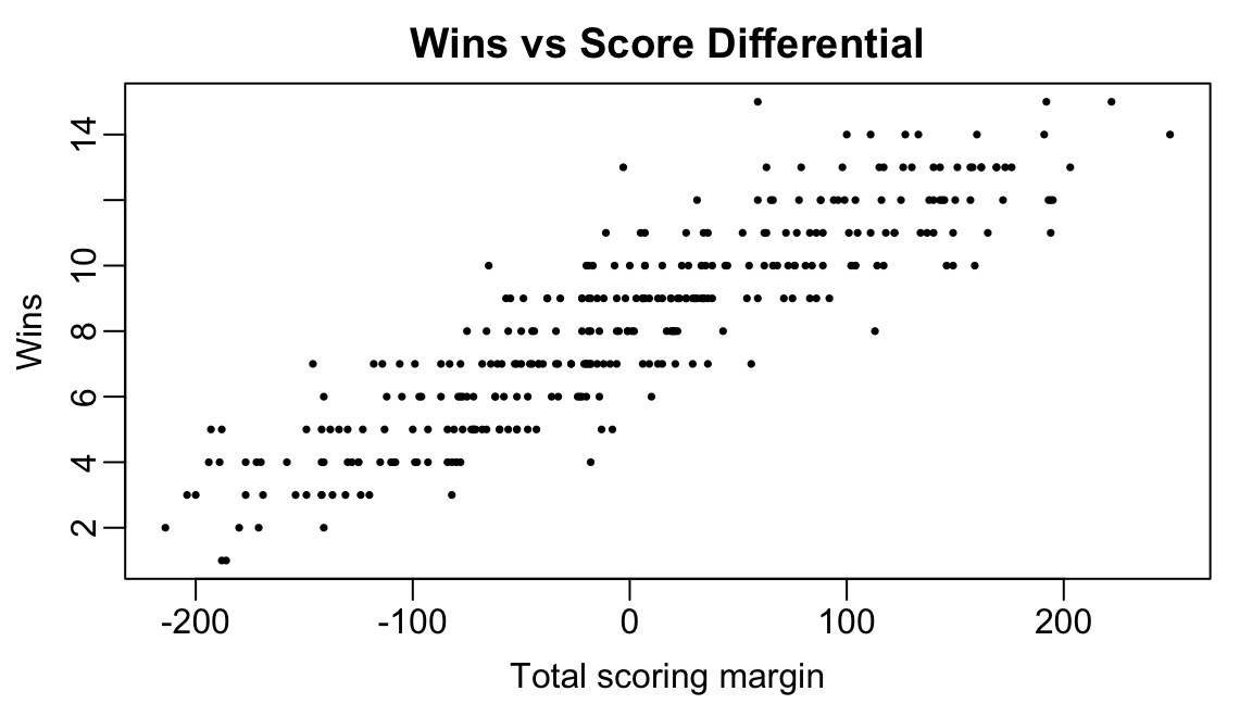
We fit a linear to these data
win_score_fit <-
  lm(wins~scoring_differential, data = records)
beta <- coefficients(win_score_fit)[2]
beta
scoring_differential
0.02807309 We see that every additional point scored is associated with about an increase of about 0.02 wins, on average.
We can now multiply each IPAR value by this factor to determine how wins each player contributes above replacement in different phases of the game.
all_skill_players <-
  unique(c(run_ipar$gsis_id, receiver_ipar$gsis_id))

skill_war <-
  data.frame(gsis_id = all_skill_players) |>
  dplyr::left_join(y = roster2024 |> dplyr::select(gsis_id, full_name, position, team), by = "gsis_id") |>
  dplyr::left_join(y = run_ipar |> dplyr::select(gsis_id, n_run, ipar_run), by = "gsis_id") |>
  dplyr::left_join(y = receiver_ipar |> dplyr::select(gsis_id, n_rec, ipar_air_rec, ipar_yac_rec), by = "gsis_id") |>
  tidyr::replace_na(list(ipar_run=0, ipar_air_rec=0, ipar_yac_rec=0)) |>
  dplyr::mutate(
    war_air_rec = ipar_air_rec * beta,
    war_yac_rec = ipar_yac_rec * beta,
    war_run = ipar_run * beta,
    war = war_air_rec + war_yac_rec + war_run)

qb_war <-
  qb_ipar |>
  dplyr::select(gsis_id, full_name, n_pass, n_qbrun, ipar_air_pass, ipar_qbrun) |>
  dplyr::left_join(y = roster2024 |> dplyr::select(gsis_id, team, position), by = "gsis_id") |>
  tidyr::replace_na(list(ipar_air_pass=0, ipar_qbrun=0)) |>
  dplyr::mutate(
    war_air_pass = ipar_air_pass * beta,
    war_qbrun = ipar_qbrun * beta,
    war = war_air_pass + war_qbrun)
Here are the top-10 skill-position players based on our WAR calculations are
skill_war |>
  dplyr::arrange(dplyr::desc(war)) |>
  dplyr::select(full_name, war) |>
  dplyr::slice_head(n=10)
full_name war
1 De'Von Achane 1.2408245
2 Saquon Barkley 1.1551989
3 Ja'Marr Chase 1.0545348
4 Jahmyr Gibbs 0.8666242
5 Jonnu Smith 0.8446721
6 Amon-Ra St. Brown 0.8086111
7 Brock Bowers 0.7438843
8 Derrick Henry 0.6381019
9 Puka Nacua 0.6084343
10 Justin Jefferson 0.6012925And here are the top-10 quarterbacks based on our WAR calculations
qb_war |>
  dplyr::arrange(dplyr::desc(war)) |>
  dplyr::select(full_name, war) |>
  dplyr::slice_head(n = 10)
# A tibble: 10 × 2
full_name war
<chr> <dbl>
1 Jayden Daniels 2.32
2 Josh Allen 2.31
3 Lamar Jackson 1.93
4 Jalen Hurts 1.72
5 Anthony Richardson 1.36
6 Brock Purdy 1.31
7 Bo Nix 1.08
8 Kyler Murray 1.05
9 Daniel Jones 0.912
10 Patrick Mahomes 0.903Exercises
- Repeat the analysis using win probability added instead of expected points added. Note,you do not need to convert from the points to win scale in this re-analysis. Which players appear to contribute the most to their team’s overall win probability?
References
Yurko, Ronald, Samuel Ventura, and Maksim Horowitz. 2019. “nflWAR: A Reproducible Method for Offensive Player Evaluation in Football.” Journal of Quantitative Analysis in Sports 15 (3): 163–83.
Footnotes
Because the vast majority of passes are thrown by quarterbacks, we’ll index passers with “q”.↩︎
Because “r” could refer to either receiver or runner, we’ll index receivers with “c” for pass catchers.↩︎
That is, unobservable.↩︎
E.g., via his route running.↩︎
If you have taken STAT 310 or 312, the issue is that the likelihood function depends on these parameters only through their sum \(\mu_{Q} + \mu_{C} + \mu_{D}.\) So, the data alone cannot distinguish configurations of these parameters that yield the same sum. For instance, setting \(\mu_{Q} = \mu_{C} = \mu_{D} = 0\) yields exactly the same fit to the data \(\mu_{Q} = 5, \mu_{C} = -5, \mu_{D} = 0.\) One way to get around this inject prior information and fit a hierarchical Bayesian model, but that is beyond the scope of this course.↩︎
The superscript \(^{(Q)}\) is there to remind us that this is for passers (i.e., quarterbacks) and the subscript \(\textrm{air}\) reminds us that the IPA values are derived from our model for EPA through the air.↩︎
In the original nflWAR paper (Yurko, Ventura, and Horowitz 2019), they set \(\Delta_{\textrm{air},i} =\Delta_{\textrm{yac},i} = \Delta_{i}\) on incomplete passes and fit the YAC EPA model using data from both complete and incomplete passes. This effectively “double counts” contributions of offensive players.↩︎
Personally, I disagree with the statement. A very natural way around this issue is to use a Bayesian hierarchical model. In fact, I’d go further and say that multilevel models of the type fitted by
lmer()are just impoverished versions of Bayesian hierarchical models. But Bayesian models are regrettably outside the scope of the course and non-Bayesian multilevel models are very widely used so you have to learn a little about them.↩︎But you should check whether our downstream results change if we estimate the YAC IPA values for receivers using a reduced model that excludes the passer random intercept!↩︎