The amount, granularity, and quality of sports data has increased exponentially over the last two decades. To draw insights and gain competitive advantages from these data, teams and leagues have invested heavily in building analytics departments. Teams are increasingly looking for analysts with the ability to ask and answer substantively interesting sports questions. Identifying such analysts is complicated by at least two factors. First, most undergraduate and graduate data science programs do not specifically train students to work with the types of data emerging in sports. And second, most of the cutting-edge data is not publicly available, making it very difficult for aspiring analysts to demonstrat their ability to analyze that data.
Public data competitions have become an increasingly popular means of identifying talent in sports analytics. Generally speaking, these competitions involve a team or league releasing a small amount of their data and inviting students and members of the public to answer substantively interesting questions using the data. The earliest competitions were hackathons organized by the NBA in the mid-2010’s1. By far the most prominent competition these days is the NFL Big Data Bowl, an annual competition in which the NFL releases a small amount of its Next Gen Stats and invites students and members of the public to use these data to draw new insight about the game. Past competitions have resulted in new ways to
Predict where a running play will end based on initial player positions (link)
Determine the optimal path for punt returners to follow (link)
Quantify the leverage created by offense when they use pre-snap motion (link)
Predict what might happen if the quarterback targeted a different receiver (link)
Big Data Bowl finalists receive a cash prize and are given a chance to present their work at the NFL Combine in Indianapolis. Over the last 8 years, over 50 people have been hired by professional teams and sports analytics companies based on their Big Data Bowl performance.
Somewhat more recently, the Connecticut Sports Analytics Symposium began organizing an open data competition specifically targeted at undergraduate and graduate students. Past competitions have involved * Determining the optimal rosters for the US Olympic gymnastics teams (link) * Determining how batter swing speed and swing length are related to batter discipline and whether pitchers can “dictate” swings (link)
In addition to presenting their work at the conference, past winners of the CSAS Data Challenge have been invited to share their finding with the US Olympic Committee.
For the third project, I would like you work with data from either the 2026 NFL Big Data Bowl or the 2026 CSAS Data Challenge. My hope is that you develop your course projects into contest submissions; the submission deadlines are December 17, 2025 for the Big Data Bowl and January 17, 2026 for the CSAS Data Challenge.
Details about both competitions and the relevant data is available below.
Big Data Bowl
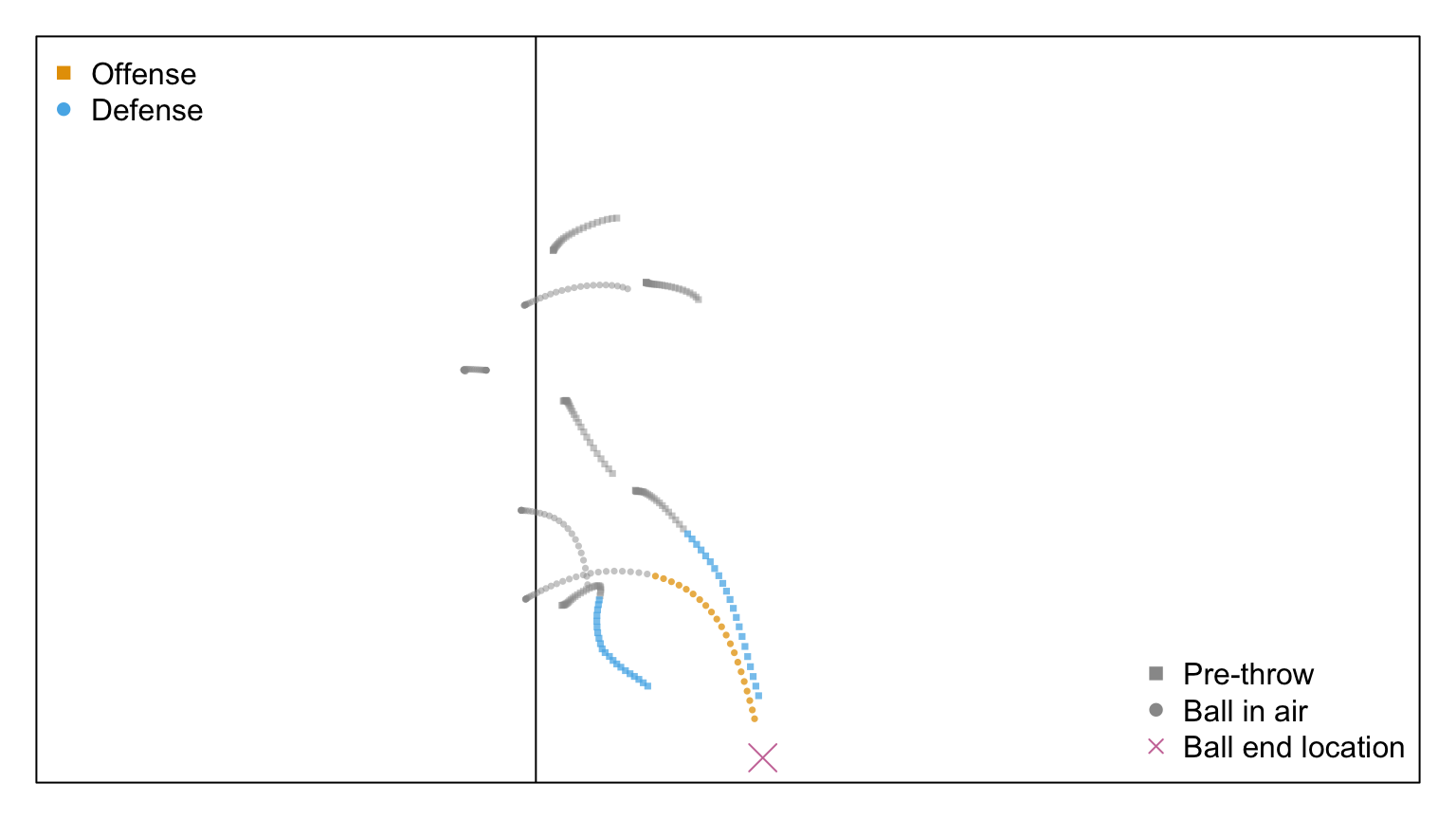
This year’s Big Data Bowl focuses on how players move during passing plays. Specifically, it tries to use tracking data between the time that the ball is snapped and the time it is thrown to predict how different players move when the ball is in the air. For the first, the NFL is running two separate competitions:
A prediction competition, in which one must predict the actual \((x,y)\) coordinates of several players at several time-steps using just their pre-throw trajectories
An analytics competition in which you must create a metric, video, or broadcast tool that helps describe player movement when the ball is in the air in a way that is accessible to coaches and fans.
For the purposes of this course, I strongly recommend focusing on the analytics competition, as it is a better opportunity to showcase your creativity and skills. The analytics competition has two tracks:
The University track: undergraduate and graduate students are tasked to analyze player movement, create player or team metrics for either the offensive or defensive players, and/or evaluate other aspects of the passing play informed by the available data
The Broadcast Visualization Track: the goal here is to create an accessible, interesting, and novel visualization that uses the movement of players when the ball in the area. For this track, participation are encouraged to overlay their visualizations over game film (available, e.g., from the NFL YouTube channel)
Data
You may download the data from the Big Data Bowl’s Kaggle website. Downloading the data from Kaggle requires registering for the competition. It is also available for download directly from this shared Box folder.
A full description of the data fields is available here. There are two CSV files for each week of the 2023 regular season. The files input_2023_w[0-18].csv contain tracking data from before the ball was thrown. Each row records where a single player is located on the field in one 0.1-second time frame2. In addition to game, play, frame, and player ID’s (game_id, play_id, frame_id and nfl_id), each row records
Information about the specific player: player_height, player_weight, player_birth_date, player_position, player_side (offense or defense), and player_role (defensive coverage, targeted receiver, passer or other route runner)
Player location and movement: their x and y coordinates, the orientation (o) and direction of player movement (dir), speed (s), acceleration (a)
Play-specific information: the yardline at the start of the play (absolute_yardline_number), where the ball lands (ball_land_x and ball_land_y)
The NFL removed tracking data for offensive and defensive linemen. They also removed data from very short passes.
Data Example
Here, we visualize a single play from the Big Data Bowl dataset. We begin by reading in data from a single week and then extracting all tracking data from a single play.
This year’s CSAS Data Challenges is about mixed double curling. In all forms of curling, teams take turns sliding stones on a sheet of ice towards a target in multiple rounds, known as “ends.” Whenever a play shoots (i.e., slides the stone), their teammates follow the stone and sweep a path along the ice with brooms to direct its motion. Teams score by having more stones closer to the center of a target than the their opponent. A considerable amount of strategy goes into shot selection: players can try to move a stone into a potential scoring position (draws); block their opponent from reaching scoring position (guards); or push already-thrown stones out of the target area (take-outs). See here for a primer on the sport.
Mixed doubles curling differs from the most common form of curling in a few important ways. First, teams consist of just two people, unlike the four-person teams in traditional curling. More substantively, at the beginning of each end in mixed doubles, two stones (one from each team) are placed in pre-determined positions along the ice: one stone will be placed within the target area and one will be placed as a guard in front of the target. In this way, one team starts with an advantage in each round.
Teams have the option to exercise a “power play” once per game during which the pre-placed stones are removed. The goal of the CSAS Data Challenge is to determine optimal strategy for the power play using data from several international competitions.
Data
The data is available for download directly from the Data Challenge GitHub. It is also available for this shared Box folder. The data is organized across multiple CSV files, which are detailed on the Data Challenge website. In addition to information about the competition and players, the data information about * The type/purpose of shot (Task) * The direction in which the stone was turned on release (Handle) * The horizontal and vertical coordinates of each stone3. * An assessment of shot quality (Points). Note this is not the number of points scored by the shot.
The data are pulled from Game Books like this one, which include images showing the locations of all stones after each shot.
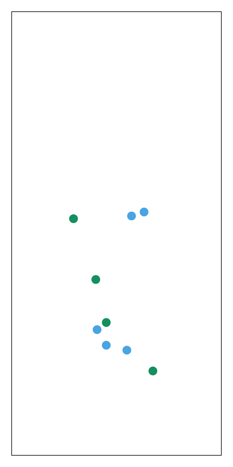
Below, we will visualize the stone locations at the conclusion of a single end in the dataset4. First, we extract all the data from a particular end in a given phase of the match, which is uniquely identified by a combination of Competition_ID, SessionID, and GameID.
The code below visualizes the locations of all stones left in play at the conclusion of a single end. Stones are colored by team.
par(mar =c(1,1,1,1), mgp =c(1.8, 0.5, 0))plot(1, type ="n", xlim =c(0,1500), ylim =c(0, 3000), xaxt ="n", yaxt ="n", xlab ="", ylab ="")for(s in1:12){ x <- tmp[10, paste0("stone_", s, "_x")] y <- tmp[10, paste0("stone_", s, "_y")]if(s <=6){if(x >0& x <4095& y >0& y <4095){points(x, y, pch =16, cex =2, col = oi_colors[3]) } } else{if(x >0& x <4095& y >0& y <4095){points(x,y, pch =16, cex =2, col = oi_colors[4]) } }}
1
Coordinates of the stone
2
The columns stone_[1-6]_x and stone_[1-6]_y are for the stones thrown by the team throwing first in the end. The columns stone_[7-12]_x and stone_[7-12]_y are for the team throwing second.
Figure 2
Potential Topics
The Data Challenge Organizers have provided a non-exhaustive list of potential topics including
The optimal time (e.g., at which score differential, in which end, etc.) to use the power play
Comparing teams’ effectiveness as using the power play and customizing strategies based on opponent tendencies
Identifying the most effective opening sequences of shots
Determining the relationship between shot quality and scoring
Deliverables
The deliverables for Project 3 are the same as for Projects and 1 & 2 and carry similar requirements.
Written Report
The written report consists of a non-technical executive summary and a technical report. The executive summary, which should not exceed 500 words, should describe the overall goals, analytic approach, and main conclusions in non-technical language. The executive summary should be free from jargon, code listings, figures, tables, and charts. It should be written to be read and understood by a front office executive, coach, player, or fan with little data science experience. The rest of written report should
Clearly state the problem being studied and provide sufficient background details and to motivate why the problem is important and interesting.
Describe the data and major steps of the analysis
Presents the main results within the context of the relevant sport(s) and supports the results with figures, tables, charts, and other statistical software output as appropriate.
Discusses the limitations of the analysis and outlines concrete steps for further development.
The technical section of the report should contain enough detail and code that another data scientist could replicate your analysis verify its soundness. Code listings and output (e.g., figures, tables, charts, and numerical summaries) should be tightly integrated with the written exposition. A good example of such integration is here. Pay particular attention to the way the author complements the numerical results with detailed examples of individual performances.
Presentation
Each team will also record an 8–10 minute presentation (e.g., using Zoom) that provides an overview of their analysis. Each presentation should include the following elements
Background (2–4 slides): clearly motivate and state the main problem being studied. Explain why it is interesting and important. Present just enough background to motivate the problem, while taking care not to overwhelm the audience with extraneous details. If appropriate, comment on the limitations of existing solutions to the problem or closely-related problems
Analysis overview (2–4 slides): present only the main steps of your analysis. Be sure to explain why each step was necessary and how these steps contribute to the overall solution. Focus more on the high-level ideas and motivation for each step rather than the specific implementation or software syntax
Main results (2–3 slides): distill your results into a few key points. Use figures, tables, charts, and other statistical software output to support your findings.
Conclusion (1 slide): briefly summarize your analysis and findings and outline between 1 and 3 specific directions for future development, improvement or refinement.
So, a single play is comprised of multiple rows.↩︎
The value 4095 is used to signal that a stone has been knocked off the sheet and the value 0 indicates that a stone has not yet been thrown.↩︎
The locations of the target circles in the given coordinate system are not immediately obvious. If you figure them out, please share on Piazza and I’ll update this page!↩︎