Lecture 5: Regularized Adjusted Plus/Minus

Overview

In Lecture 4, we introduced adjusted plus/minus, which attempts to estimate how much value an NBA player creates after adjusting for the quality of his teammates and opponents. As noted in that lecture, using the method of least squares to estimate APM values is problematic because it assumes that all baseline players have the exact same partial effect on their team’s average point differential per 100 possessions. In this lecture, we solve a penalized version of the least squares problem (Section 2) to fit a regularized adjusted plus/minus model that avoids the need to specify baseline players (Section 3). We then use the bootstrap (Section 4) to quantify uncertainty about differences between players and the overall RAPM rankings.

Notation Review

We begin by reviewing the notation and set-up from Lecture 4. First, let \(n\) denote the number of stints and \(p\) the total number of players. For each stint \(i = 1, \ldots, n\) and player \(j = 1, \ldots, p,\) let \(x_{ij}\) be the signed on-court indicator for player \(j\) during stint \(i.\) That is, \(x_{ij} = 1\) (resp. \(x_{ij} = -1)\) if player \(j\) is on the court and playing at home (resp. on the road) during stint \(i\) and \(x_{ij} = 0\) if player \(j\) is not on the court during stint \(i.\) We can arrange these indicators into a large \(n \times p\) matrix \(\boldsymbol{\mathbf{X}}\) whose rows (resp. columns) correspond to stints (resp. players). Finally, let \(Y_{i}\) be the point differential per 100 possessions observed during shift \(i.\)

The original APM model introduced a single number \(\alpha_{j}\) for each player \(j = 1, \ldots, p,\) and modeled \[ \begin{align} Y_{i} &= \alpha_{0} + \alpha_{h_{1}(i)} + \alpha_{h_{2}(i)} + \alpha_{h_{3}(i)} + \alpha_{h_{4}(i)} + \alpha_{h_{5}(i)} \\ ~&~~~~~~~~~~- \alpha_{a_{1}(i)} - \alpha_{a_{2}(i)} - \alpha_{a_{3}(i)} - \alpha_{a_{4}(i)} - \alpha_{a_{5}(i)} + \epsilon_{i}, \end{align} \] where \(h_{1}(i), \ldots, h_{5}(i)\) and \(a_{1}(i), \ldots, a_{5}(i)\) are, respectively, the indices of the homes and away team players on the court during stint \(i\); \(\alpha_{0}\) captures the average home court advantage in terms of point-differential per 100 possessions across all teams; and the \(\epsilon_{i}\)’s are independent random errors drawn from a distribution with mean zero.

In Lecture 4, we formed the \(n \times (p+1)\) matrix \(\boldsymbol{\mathbf{Z}}\) by appending a column of 1’s to the matrix \(\boldsymbol{\mathbf{X}}\) and let \(\boldsymbol{\alpha} = (\alpha_{0}, \alpha_{1}, \ldots, \alpha_{p})^{\top}\) be the vector of length \(p+1\) containing the home court advantage \(\alpha_{0}\) and all the player-specific parameters \(\alpha_{j}.\) Letting \(\boldsymbol{\mathbf{z}}_{i}\) be the \(i\)-th row of \(\boldsymbol{\mathbf{Z}},\) we can write the APM model in a more compact form. \[ Y_{i} = \boldsymbol{\mathbf{z}}_{i}^{\top}\boldsymbol{\alpha} + \epsilon_{i}. \]

At the end of Lecture 4, we saved a copy of the full matrix \(\boldsymbol{\mathbf{X}}\) (which we called X_full) of signed on-court indicators, a vector of point differentials per 100 possessions \(\boldsymbol{Y}\) (Y), and a look-up table containing player id numbers and names. We load those objects into our environment.

load("lecture04_05_data.RData")

Ridge Regression

Unfortunately, a unique least squares estimator of \(\boldsymbol{\alpha}\) does not exist. This is because the matrix \(\boldsymbol{\mathbf{Z}}^{\top}\boldsymbol{\mathbf{Z}}\) does not have a unique inverse[^rankdeficient]. Instead, there are infinitely many different vector \(\boldsymbol{\alpha}\) that minimize the quantity \[ \sum_{i = 1}^{n}{(Y_{i} - \boldsymbol{\mathbf{z}}_{i}^{\top}\boldsymbol{\alpha})^{2}}, \] Complicating matters further, the data do not provide any guidance from picking between these minimizers as they all yield the same sum of squared errors. The original developers of adjusted plus/minus overcame this issue by (i) specifying a group of baseline-level players; (ii)

Rather than minimize the sum of the squared errors, we will instead try to minimize the quantity \[ \sum_{i = 1}^{n}{(Y_{i} - \boldsymbol{\mathbf{z}}_{i}^{\top}\boldsymbol{\alpha})^{2}} + \lambda \times \sum_{j = 0}^{p}{\alpha_{j}^{2}}, \] where \(\lambda > 0\) is a fixed number¹.

The first term is the familiar sum of squared errors \(\sum{(Y_{i} - \boldsymbol{\mathbf{z}}_{i}^{\top}\boldsymbol{\alpha})^{2}}.\) The second term \(\sum_{j}{\alpha_{j}^{2}}\) is known as the shrinkage penalty because it is small whenever all the \(\alpha_{j}\)’s are close to zero (i.e., when they are shrunk towards zero). Minimizing the penalized sum of squares trades off finding \(\alpha_{j}\)’s that best fit the data (i.e., minimize the squared error) and finding \(\alpha_{j}\)’s that are not too far away from zero. When \(\lambda\) is very close to zero, the shrinkage penalty tends to exert little influence but as \(\lambda \rightarrow \infty,\) the penalty dominates and the minimizer converges to the vector of all zeros. Consequently, it is imperative that we select a good value of \(\lambda.\)

Before discussing how we set the tuning parameter \(\lambda\) in practice, it is worth pointing out that for every \(\lambda > 0,\) a unique solution to the penalized sum of squares problems exists and is available in closed-form: \[ \hat{\boldsymbol{\alpha}}(\lambda) = \left(\boldsymbol{\mathbf{Z}}^{\top}\boldsymbol{\mathbf{Z}} + \lambda I \right)^{-1}\boldsymbol{\mathbf{Z}}^{\top}\boldsymbol{\mathbf{Y}}, \] Looking at this formula, we notice that the expression is very nearly identical to the general formula for ordinary least squares. The only difference is that we’ve added \(\lambda\) to the diagonals of \(\boldsymbol{\mathbf{Z}}^{\top}\boldsymbol{\mathbf{Z}}\), which guarantees that the matrix \(\boldsymbol{\mathbf{Z}}^{\top}\boldsymbol{\mathbf{Z}} + \lambda I\) has a unique inverse. This technique of adding a small perturbation to \(\boldsymbol{\mathbf{Z}}^{\top}\boldsymbol{\mathbf{Z}}\) in the least squares formula — which is equivalent to solving the penalized sum of squares problem — is known as ridge regression.²

Picking \(\lambda\) with Cross-Validation

In practice, we typically pick a value of \(\lambda\) using cross-validation The basic idea is to select the value of \(\lambda\) that results in the smallest out-of-sample prediction error. Since we don’t have any out-of-sample data, we will instead approximate it using the technique from Lecture 3 in which we repeatedly held out a subset of the data when training our model and then assessed the error on the held-out data. This process is known as “cross-validation.”

More specifically, we begin by specifying a large grid of potential \(\lambda\) values. Then, for each \(\lambda\) in the grid, we repeatedly iterate through the following steps. 1. Form a random training/testing split 2. Fit a ridge regression model with the current value of \(\lambda\) using only the training subset to obtain an estimate \(\hat{\boldsymbol{\alpha}}(\lambda)\) 3. Compute the average of the squared errors \(\left(Y_{i} - \boldsymbol{\mathbf{z}}_{i}^{\top}\hat{\boldsymbol{\alpha}}(\lambda) \right)\) in the testing subset. After iterating through these steps many times for a single \(\lambda,\) we compute the average out-of-sample errors (across the different training/testing splits) before moving onto the next \(\lambda\) value in the grid.

At the end of this process, we have an estimate for the out-of-sample mean square error for every \(\lambda\) and can pick the \(\lambda\) that yields the smallest one. Then, we can fit a ridge regression model using all of the data to obtain our final solution.

Regularized Adjusted Plus/Minus

To recap, by fitting a ridge regression model instead of an ordinary linear model, we are able to estimate an adjusted plus/minus value for all players, thereby avoiding having to specify an arbitrary baseline-level. Although this is conceptually easy, finding a suitable \(\lambda\) via cross-validation is quite an involved process. Luckily for us, the function cv.glmnet() from the glmnet package automates the process (including specifying the initial grid).

The following code shows how to perform the cross-validation, plots the cross-validation error for each value of \(\lambda\), and selects the \(\lambda\) with smallest error.

set.seed(479)
library(glmnet)
cv_fit <-
  cv.glmnet(x = X_full, y = Y,
            alpha = 0,
            standardize = FALSE)
lambda_min <- cv_fit$lambda.min

1: Because cross-validation involves forming random training/testing splits, setting the randomization seed ensures our results are reproducible.
2: Load the glmnet package into our R environment
3: Unlike lm, glmnet functions do not use a formula argument. Instead, you must manually pass the design matrix (without intercept) and output vector.
4: The argument alpha = 0 tells glmnet to use a squared error penalty.
5: It is extremely important to set standardize = FALSE. If you don’t, you end up over-shrinking the APM estimates of players with lots of playing time and under-shrinking APM estimates for players with little playing time
6: Extracts the value of \(\lambda\) with smallest out-of-sample error

We can plot the out-of-sample error as a function of \(\lambda\):

par(mar = c(3,3,2,1), mgp = c(1.8, 0.5, 0))
plot(cv_fit)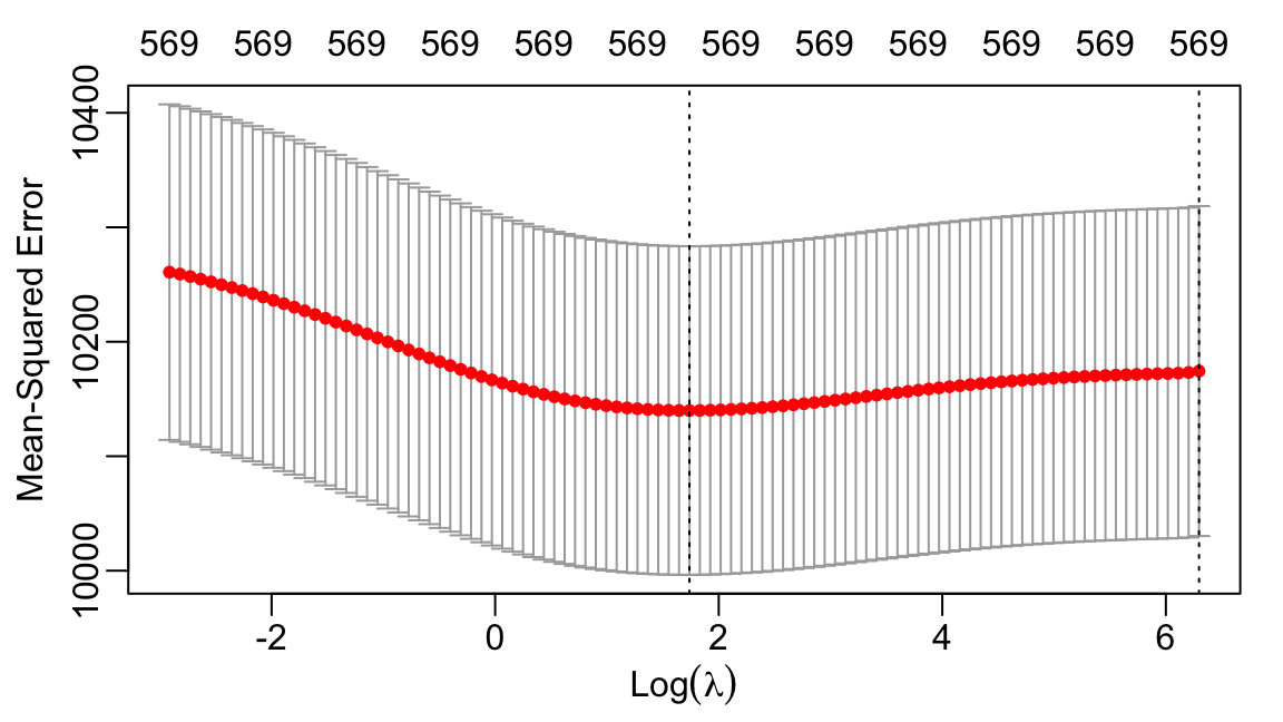

Plots the out-of-sample error as a function of \(\lambda.\)

We can now fit a ridge regression model with the cross-validated choice of \(\lambda\) using data from all our stints. Because we do not need to run cross-validation again, we use the function glmnet instead of cv.glmnet.

In the following code, we actually fit a ridge regression model using all values of \(\lambda\) from the grid constructed by cv.glmnet(). This is because the function glmnet can behave a little strangely when only one value of \(\lambda\) is specified³. Then, we pull out the estimated coefficients corresponding to the optimal \(\lambda\) value.

lambda_index <- which(cv_fit$lambda == lambda_min)
fit <-
  glmnet(x = X_full, y = Y,
         alpha = 0,
         lambda = cv_fit$lambda,
         standardize = FALSE)

alpha_hat <- fit$beta[,lambda_index]

rapm <-
  data.frame(
    id = names(alpha_hat),
    rapm = alpha_hat) |>
  dplyr::inner_join(y = player_table |> dplyr::select(id,Name), by = "id")

1: Determines where in the grid of \(\lambda\) values specified by cv_glmnet() the optimal one lies.
2: Solves the ridge regression problem at all values of \(\lambda\) along the grid specified by the initial cv_glmnet() fit.
3: glmnet() returns a matrix of parameter estimates where the columns correspond to the different \(\lambda\) values. Here, we pull out the estimates for the optimal \(\lambda\), which was the second value provided.
4: Like we did in Lecture 4, we create a data frame with every players’ regularized adjusted plus/minus value and name

We recognize many super-star-level players (e.g., Gilgeous-Alexander, Dončić, Jokić, Giannis) among those with the highest regularized adjusted plus/minus values.

rapm |>
  dplyr::arrange(dplyr::desc(rapm)) |>
  dplyr::slice_head(n = 10)

        id     rapm                    Name
1  1628983 3.602143 Shai Gilgeous-Alexander
2  1627827 3.472249     Dorian Finney-Smith
3  1630596 3.415232             Evan Mobley
4  1629029 3.352736             Luka Doncic
5   202699 3.183716           Tobias Harris
6   203999 2.846327            Nikola Jokic
7  1631128 2.829463         Christian Braun
8  1628384 2.813794              OG Anunoby
9   203507 2.646488   Giannis Antetokounmpo
10 1626157 2.641075      Karl-Anthony Towns

Recall that in our regularized adjusted plus/minus model, the individual \(\alpha_{j}\)’s correspond to a somewhat absurd counter-factual. Specifically, \(\alpha_{j}\) represents the amount by which a team’s point differential per 100 possession increases if they go from playing 4-on-5 to playing 5-on-5 with player \(j\) on the court. Differences of the form \(\alpha_{j} - \alpha_{j'}\) are much more useful than the single \(\alpha_{j}\) values. By replacing player \(j'\) with player \(j,\) a team can expect to score \(\alpha_{j} - \alpha_{j'}\) more points per 100 possessions.

For instance, by replacing Luka Dončić with Anthony Davis, teams are expected to score an additional -3.41 points per possession⁴.

luka_rapm <- rapm |> dplyr::filter(Name == "Luka Doncic") |> dplyr::pull(rapm)
ad_rapm <- rapm |> dplyr::filter(Name == "Anthony Davis") |> dplyr::pull(rapm)

ad_rapm - luka_rapm

[1] -3.417006

Uncertainty Quantification with the Bootstrap

So far, we have only focused on obtaining point estimates. What is the range of our uncertainty about the relative impact of players.

The bootstrap is an elegant way to quantify uncertainty about the output particular statistical method. At a high-level, the bootstrap works by repeatedly sampling observations from the original dataset and applying the method to the re-sampled dataset. In the context of our RAPM analysis, we will repeat the following steps many, many times (e.g., \(B = 100\) times):

Randomly draw a sample of \(n\) stints with replacement
Using the random re-sample, compute an estimate of the RAPM parameters \(\hat{\boldsymbol{\alpha}}(\hat{\lambda})\) by fitting a ridge regression model with the optimal \(\lambda\) found by our initial cross-validation.
Save the estimates in an array

Running this procedure, we obtain \(B\) different estimates \(\hat{\boldsymbol{\alpha}}(\lambda)^{(1)}, \ldots, \hat{\boldsymbol{\alpha}}(\lambda)^{(B)}\) where \(\hat{\boldsymbol{\alpha}}(\lambda)^{(b)}\) is the estimate obtained during the \(b\)-th time through the loop. Importantly, each bootstrap estimate of the whole vector \(\boldsymbol{\alpha}\) yields a bootstrap estimate of the constrast \(\alpha_{j} - \alpha_{j'}.\) By examining the

As a concrete illustration, the following code computes 500 bootstrap estimates of the RAPM parameter vector. It saves the bootstrap estimates of \(\boldsymbol{\alpha}\) in a large matrix whose rows correspond to bootstrap samples and whose columns correspond to players.

Important

##Warning The following code takes several minutes to run!

B <- 500
n <- nrow(X_full)
p <- ncol(X_full)
player_names <- colnames(X_full)
boot_rapm <- 
  matrix(nrow = B, ncol = p,
         dimnames = list(c(), player_names))

for(b in 1:B){
  if(b %% 10 == 0) cat(b, " ")
  set.seed(479+b)
  boot_index <- sample(1:n, size = n, replace = TRUE)
  
  fit <- 
    glmnet(x = X_full[boot_index,], y = Y[boot_index],
           alpha = 0,
           lambda = cv_fit$lambda,
           standardize = FALSE)
  tmp_alpha <- fit$beta[,lambda_index]
  boot_rapm[b, names(tmp_alpha)] <- tmp_alpha
}

1: Set number of bootstrap iterations
2: Get the number of stints and players
3: Get the list of player id’s, which are also the column names of X_full
4: Build a \(B \times p\) matrix to store bootstrap estimates of \(\boldsymbol{\alpha}.\)
5: Use the players’ IDs as column names for boot_rapm
6: We set the seed for reproducibility. But we need to vary the seed with every bootstrap re-sample. Otherwise, we’d be drawing the exact same sample every time!
7: This is a list of row-indices for our re-sampled stints.
8: Takes advantage of R’s indexing capabilities to create our re-sampled design matrix and outcome vector
9: Saves the bootstrap estimate of \(\boldsymbol{\alpha}\) in the \(b\)-th row of boot_ramp

10  20  30  40  50  60  70  80  90  100  110  120  130  140  150  160  170  180  190  200  210  220  230  240  250  260  270  280  290  300  310  320  330  340  350  360  370  380  390  400  410  420  430  440  450  460  470  480  490  500

We can now compute the difference between Dončić’s and Davis’ estimated RAPM values for every bootstrap estimate. We find that the overwhelming majority of these samples are negative, suggesting that that we can be virtually certain that a team is expected to score score fewer points per 100 possessions by replacing Dončić by Davis.

doncic_id <- player_table |> dplyr::filter(Name == "Luka Doncic") |> dplyr::pull(id)
davis_id <- player_table |> dplyr::filter(Name == "Anthony Davis") |> dplyr::pull(id) 

boot_diff <- boot_rapm[,davis_id] - boot_rapm[,doncic_id]

hist(boot_diff,
     breaks = 20,
     main = "Bootstrap Distribution of Davis-Doncic", 
     xlab = "Difference")

1: Get Dončić’s and Davis’ ids
2: Get the vectors of Dončić’s and Davis’ bootstrapped RAPM values by extracting the relevant columns from boot_rapm and compute the difference
3: Make a histogram of the bootstrapped differences between Davis’ and Dončić’s RAPM values
4: Set the number of bins in the histogram to 20

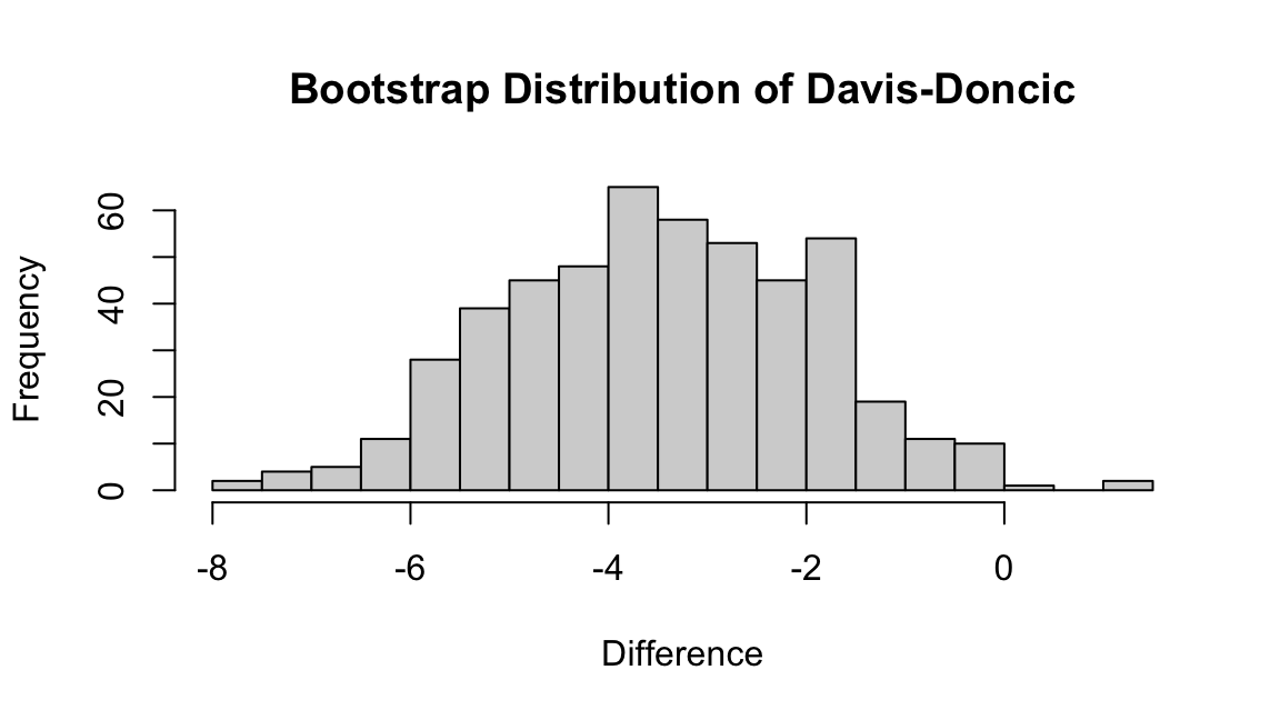
Figure 2: Bootstrap distribution of difference between Doncic & Davis

We can form an uncertainty interval using the sample quantiles of the bootstrapped differences between Davis’ and Dončić’s RAPM values.

quantile(boot_diff, probs = c(0.025, 0.975))

1: A 95% uncertainty interval can be formed using the 2.5% and 97.5% quantiles of the bootstrapped estimates

      2.5%      97.5% 
-6.3776674 -0.4839716

We conclude with 95% confidence that by replacing Dončić by Davis, the Mavericks are expected to score between 0.48 and 6.3 fewer points per 100 possessions.

Bootstrap Intervals for Ranks

Recall that in our original analysis, Shai Gilgeous-Alexander had the highest RAPM value. How certain should we be about his overall ranking?

Just like we computed the difference between Dončić’s and Davis’ RAPM estimates for every bootstrap re-sample, we can compute the rank of SGA’s RAPM estimate in every bootstrap sample. Then, we can look at the bootstrap distribution of these ranks to get an idea about the uncertainty in the rank.

The rank() function returns the sample ranks of the values in vector. For instance,

x <- c(100, -1, 3, 2.5, -2)
rank(x)

[1] 5 2 4 3 1

Notice that the smallest value in x (-2) is ranked 1 and the largest value in x (100) is ranked 5. This demonstrates that rank() assigns ranks in increasing order. If we wanted the largest value to be ranked 1, the second largest ranked 2, etc., then we need to call rank on the negative values:

rank(-x)

[1] 1 4 2 3 5

The following code confirms that SGA ranked first in terms of the original RAPM estimate.

rapm <-
  rapm |>
  dplyr::mutate(rank_rapm = rank(-1 * rapm))

rapm |> dplyr::filter(Name == "Shai Gilgeous-Alexander")

       id     rapm                    Name rank_rapm
1 1628983 3.602143 Shai Gilgeous-Alexander         1

To quantify the uncertainty in SGA’s RAPM ranking, we need to rank the values within every bootstrap estimate of \(\boldsymbol{\alpha}.\) In other words, we need to rank the values within every row of boot_rapm. We can do this using the apply() function. For our purposes, apply() runs a function (specified using the FUN argument) on every row or column of a two-dimensional array. To run the function along every row, one specifies the argument MAR = 1 and to run the function along every column, one specifies the argument MAR = 2. Notice that the output has \(p\) rows (one for every player) and \(B\) columns (one for every bootstrap iteration).

boot_rank <- 
  apply(-1*boot_rapm, MARGIN = 1, FUN = rank)
dim(boot_rank)

[1] 569 500

To get the bootstrap distribution of SGA’s ranking, we need to extract the values from the corresponding row of boot_rank. In the following code, we first look up SGA’s player ID and then get the values from the row of boot_rank that is named with SGA’s ID.

sga_id <- 
  player_table |>
  dplyr::filter(Name == "Shai Gilgeous-Alexander") |>
  dplyr::pull(id)

sga_ranks <- boot_rank[sga_id,]
table(sga_ranks)

sga_ranks
  1   2   3   4   5   6   7   8   9  10  11  12  13  14  16  17  18  19  20  21 
 58  59  46  55  36  21  19  12  17  17  13  10   8  12   8   5   2   9   6   5 
 22  23  24  25  26  27  28  29  30  31  32  33  34  36  37  38  39  40  41  44 
  4   5   4   5   5   2   2   4   5   2   2   5   4   3   2   1   2   1   1   2 
 45  47  48  51  52  56  57  66  70  84  85  86  91 105 106 176 
  5   1   1   1   1   2   1   1   1   1   1   1   1   1   1   1

It turns out that SGA had the highest RAPM value in just 58 of our 500 bootstrap samples and the second-highest RAPM value in 59 of our bootstrap samples. We can form a 95% bootstrap uncertainty interval around his overall ranking by computing the sample quantiles of these rankings.

quantile(sga_ranks, probs = c(0.025, 0.975))

  2.5%  97.5% 
 1.000 51.525

Our analysis reveals quite a bit of uncertainty about SGA’s overall rank in terms of RAPM!

Exercises

Pick several players and compare the bootstrap distribution of the difference in their RAPM estimates.
Using the same 100 training/testing splits constructed in Exercise 4.5, estimate the out-of-sample mean square error for RAPM based on the 2024-25 data. Instead of computing an optimal \(\lambda\) for each training split, you may use the optimal \(\lambda\) value computed on the whole dataset. Is RAPM a better predictive model than APM?
Fit RAPM models to data from (i) the 2023-24 and 2024-25 regular seasons and (ii) the 2022-23, 2023-24, and 2024-25 regular season. Use the bootstrap to quantify how uncertainty about the difference in player RAPM values and the overall rankings changes as you include data from more seasons.
Just like lm, the functions cv.glmnet() and glmnet() accept a weights argument. Using the weighting schemes you considered in Exercise 4.2, fit regularized weighted adjusted plus/minus models.

Footnotes

In practice, \(\lambda\) is often determined using the data. See Section 2.1.↩︎
See Section 6.2 of An Introduction to Statistical Learning for a good review of ridge regression.↩︎
In fact, the glmnet() documentation explicitly warns users from running with only a single value of \(\lambda.\)↩︎
Once again: Fire Nico.↩︎