Lecture 13: Tournament Simulation

Overview

In Lecture 12, we used a Bradley-Terry model to estimate the latent strength of each Division I women’s ice hockey team. The model posits that the log-odds of one team beating the other is simply the difference in these latent strengths. According to our model estimates, the Wisconsin Badgers and Ohio State Buckeyes were ranked 1st and 2nd among all teams. Using the estimated model parameters, we simulated a “best-of-5” series between the two teams, finding that Wisconsin was predicted to win such a series about 91% of the time.

One major drawback of our initial model is that it fails to account for any potential home-court advantage. In other words, it assumes that the probability that Wisconsin beats Ohio State is the same whether the game was played at La Bahn Arena (the home of the Wisconin Badgers), the Ohio State University Ice Rink, or at a neutral site.

In this lecture, we fit a refined version of the Bradley-Terry model that accounts for location. We introduce this model in Section 2 and perform the necessary pre-processing in Section 3. Then, in Section 4, we fit the model using the BradleyTerry2 package and examine the resulting power rankings. Finally, in Section 5 we simulate the semi-finals and finals of the 2025 NCAA Tournament under several different scenarios.

Before proceeding, we load in the data table containing all regular season Division I women’s ice hockey games from the 2024-25 season that did not end in ties.

load("wd1hockey_regseason_2024_2025.RData")

Bradley-Terry Models with Home-Court Advantage

Like the basic model from Lecture 12, we will associate a latent parameter \(\lambda_{j}\) to each team \(j = 1, \ldots, p.\) We will also fix one \(\lambda_{j} = 0\), corresponding to a pre-specified reference team¹. In addition to the latent team strengths \(\lambda_{1}, \ldots, \lambda_{p},\) we will introduce an additional parameter \(\lambda_{0}\) that accounts for a systematic home advantage.

Now suppose that the home team \(H\) plays an away team \(A\) at team \(H\)’s home. Our augmented Bradley-Terry model asserts that the log-odds that \(H\) beats \(A\) is \(\lambda_{0} + \lambda_{H} - \lambda_{A}.\) Equivalently, our augmented model asserts that \[ \mathbb{P}(\textrm{team H beats team A at H's home}) = \frac{e^{\lambda_{H} + \lambda_{0}}}{e^{\lambda_{H} + \lambda_{0}} + e^{\lambda_{A}}}. \] Compared to the original Bradley-Terry model we considered in Lecture 12, our new model gives a systematic advantage to the home team. For any two teams \(i\) and \(j,\) our original Bradley-Terry model assumes that the probability of team \(i\) beating team \(j\) is the same across all locations. Under our new model, the model makes a different prediction depending on location: the log-odds of \(i\) beating \(j\) are

\(\lambda_{0} + \lambda_{i} - \lambda_{j}\): if the game is played at \(i\)’s home arena
\(-\lambda_{0} + \lambda_{i} - \lambda_{j}\): if the game is played at \(j\)’s home arena
\(\lambda_{i} - \lambda_{j}\): if the game is played at a neutral site (i.e., not at \(i\)’s or \(j\)’s home arena)

To derive the log-odds of \(i\) beating \(j\) at \(j\)’s home arena, note that according to our model \[ \mathbb{P}(\textrm{team j beats i at j's home}) = \frac{e^{\lambda_{j} + \lambda_{0}}}{e^{\lambda_{j} + \lambda_{0}} + e^{\lambda_{i}}}. \] Thus \[ \begin{align} \mathbb{P}(\textrm{team i beats j at j's home}) &= \frac{e^{\lambda_{i}}}{e^{\lambda_{j} + \lambda_{0}} + e^{\lambda_{i}}} \\ &= \frac{1}{e^{\lambda_{j} + \lambda_{0} - \lambda_{i}} + 1} \\ &= \frac{1}{1 + e^{-1 \times (-\lambda_{0} + \lambda_{i} - \lambda_{j})}}. \end{align} \]

Data Preparation

Unfortunately, the data table we scraped from USCHO does not record the location of the game. USCHO publishes box scores for individual games on separate webpages with highly structured URLs. For instance, the URL for the webpage with the box score from the championship game between the Badgers and Buckeyes is

https://www.uscho.com/gameday/division-i-women/2024-2025/2025-03-23/game-7949/

Notice that after the date there is a unique game identifier (7949 in this case). Based on this, it is tempting to write a function that visits each individual site (e.g., by looping over the unique game ID’s). Unfortunately, this strategy requires us to determine the unique game identifiers, which is not entirely straightforward. We instead manually impute the location information with some heuristics.

Determining Location

We will assume all non-tournament conference games and most tournament games are played at the home arena of the listed home team and not at a neutral site. For instance, there were four games in Icebreaker tournament featured four games:

Penn State vs Cornell (boxscore)
Stonehill vs Ohio State (boxscore)
Cornell vs Ohio State (boxscore)
Stonehill vs Penn State (boxscore)

no_ties |>
  dplyr::filter(grepl("IceBreaker", Notes)) |>
  dplyr::select(Date, Opponent, Home, Notes, Type)

# A tibble: 4 × 5
  Date       Opponent   Home       Notes      Type 
  <chr>      <chr>      <chr>      <chr>      <chr>
1 10/25/2024 Penn State Cornell    IceBreaker NC   
2 10/25/2024 Stonehill  Ohio State IceBreaker NC   
3 10/26/2024 Cornell    Ohio State IceBreaker NC   
4 10/26/2024 Stonehill  Penn State IceBreaker NC

Inspecting the box scores pages for all four games, we see that they were all played at Value City Arena. Although this is located at the Ohio State University — and is the home arena of their men’s ice hockey team — it is not the home arena of the women’s ice hockey team. For the purposes of our analysis, we will assume that the games in this tournament are played at a neutral site.

To record whether the game was played at the home arena of Home or at a neutral site, we will first identify all tournaments by pulling out the unique values in Notes that do not include the string "SO".

unik_notes <-
  no_ties |>
  dplyr::filter(!is.na(Notes) & !grepl("SO", Notes)) |>
  dplyr::pull(Notes) |>
  unique()
unik_notes

 [1] "IceBreaker"          "Nutmeg Classic"      "Smashville Showcase"
 [4] "Mayor's Cup"         "East/West Classic"   "Beanpot"            
 [7] "ECAC Tournament"     "AHA Tournament"      "HEA Tournament"     
[10] "WCHA Tournament"     "NEWHA Tournament"

We then manually inspect the box scores for each of the tournaments to determine whether they were played at any of the team’s home arena. We find * The East/West Classic was played at Ridder Arena, which is the home arena of Minnesota. So, we will treat the the games between Penn State and Bemidji State and between Brown and Bemidji State as being played at a neutral site. But we will treat the games involving Minneosta as being played at their home arena. * The Nutmeg Classic was played at Martire Family Arena, which is the home arena of Sacred Heart. So, we will treat games from this tournament that do not involve Sacred Heart can be considered a neutral site game. * The Mayor’s Cup game between Brown and Providence was played at Schneider Arena, which is the home arena of Providence. * The Mayor’s Cup game between Union and RPI was played at MVP Arena, which is a neutral site * All games in the Smashville Showcase were played at a neutral site: they were played at the Ford Ice Center, which is not the home arena of any of St. Thomas, Merrimack, Clarkson, or Penn State. * The Beanpot games between Boston University and Harvard and Boston College and Northeastern were played at Matthews Arena, which is the home arena of Northeastern. The games between Boston College and Harvard and Boston University and Northeastern were played at the T.D. Garden, which is a neutral site.

Generally speaking, most conference tournament games were played at the home arena of the listed home team. We find that:

All games in the NEWHA, and AHA, and HEA tournaments were played at the higher-ranked seeds home arena. So, none of these tournament games were played at a neutral site.
All but the last three games of the ECAC tournament were held at the listed home team’s home arena. The last three games (St. Lawrence vs Colgate, Clarkson vs Cornell, and Colgate vs Cornell) were held at Cornell’s home arena. So only the March 7, 2025 game between St. Lawrence and Colgate was held at a neutral site.
All the but last three games of the WHCA tournament were held at the listed home team’s home arena. The last three (Minnesota vs Ohio State State, Minnesota Duluth vs Wisconsin, and Minnesota vs Wisconsin) were held at Minneosta Duluth’s home arena. So, the March 7, 2025 game between Minnesota and Ohio State and the March 8, 2025 game between Minnesota and Wisconsin were held at a neutral site.

Based on these findings, we create a new variable in no_ties, which records whether the game was played at a neutral site.

no_ties <-
  no_ties |>
  dplyr::mutate(
    neutral = dplyr::case_when(
      grepl("IceBreaker", Notes) ~ 1,
      grepl("East/West", Notes) & Home != "Minnesota" ~ 1,
      grepl("Nutmeg", Notes) & Home != "Sacred Heart" ~ 1,
      grepl("Mayor", Notes) & Home == "Rensselaer" ~ 1,
      grepl("Smashville", Notes) ~ 1,
      grepl("Beanpot", Notes) & Home != "Northeastern" ~ 1, 
      Date == "3/7/2025" & Home == "St. Lawrence" & Opponent == "Colgate" ~ 1,
      Date == "3/7/2025" & Home == "Minnesota" & Opponent == "Ohio State" ~ 1,
      Date == "3/8/2025" & Home == "Minnesota" & Opponent == "Wisconsin" ~ 1,
      .default = 0))

Fitting Our Model

Recall from Lecture 12 that we counted up the number of home and away team wins for every unique combination of home and away teams. Because we now wish to account for potential home advantages, we need to separate these counts based on the game location. To do this, we will subdivide the games in no_ties based on the combination of Home, Opponent, and neutral and count up the numbers of home and away team wins. In the code below, we also rename Home and Opponent.

unik_teams <- sort(unique(c(no_ties$Home, no_ties$Opponent)))

results <-
  no_ties |>
  dplyr::rename(home.team = Home, away.team = Opponent) |>
  dplyr::group_by(home.team, away.team, neutral) |> 
  dplyr::summarise(
    home.win = sum(Home_Winner), 
    away.win = sum(Opp_Winner), .groups = 'drop') |> 
  dplyr::mutate(
    home.team = factor(home.team, levels = unik_teams), 
    away.team = factor(away.team,levels = unik_teams),
    home.athome = ifelse(neutral == 1, 0, 1),
    away.athome = 0)

1: This is a bit redundant but is necessary to set up the call to BTm().

Fitting our more elaborate Bradley-Terry model requires somewhat more complicated syntax. Following the example from Section 3.3 of the package vignette “Bradley-Terry Models in R”, we create a temporary data frame tmp_df containing the numbers of home and away team wins for every combination of home.team, away.team, and neutral. We then add two more columns to this data frame, one for the home team (home.team) and one for the away team (away.team). These columns are themselves data frames² with columns recording team identity and whether the team was playing at home.

tmp_df <- data.frame(home.win = results$home.win, away.win = results$away.win)
tmp_df$home.team <- data.frame(team = results$home.team, at.home = results$home.athome)
tmp_df$away.team <- data.frame(team = results$away.team, at.home = results$away.athome)

fit <-
  BradleyTerry2::BTm(
    outcome = cbind(home.win, away.win),
    player1 = home.team, player2 = away.team,
    formula = ~ team + at.home,
    refcat = "New Hampshire",
    id = "team",
    data = tmp_df)

1: BTm uses a somewhat non-standard formula interface. This specification tells BTm() to estimate a separate latent strength for each team and a parameter for the home advantage.
2: Manually specify the reference team (whose \(\lambda\) is set to 0)
3: The id argument specifies that “team” is the name of the factor used to identity teams

Inspecting the model parameters, we see \(\hat{\lambda}_{0} \approx 0.311.\) A change of this magnitude on the log-odds scale corresponds to a change of

26% (log-odds of -1) to 33% (log-odds of -0.689)
46% (log-odds of -0.156) to 54% (log-odds of 0.156)
73% (log-odds of 1) to 79% (log-odds of 1.311)

round(coef(fit), digits = 3)

       teamAssumption     teamBemidji State    teamBoston College 
               -4.746                -0.753                 0.885 
teamBoston University             teamBrown          teamClarkson 
                1.135                 0.150                 1.225 
          teamColgate       teamConnecticut           teamCornell 
                2.075                 1.118                 2.636 
        teamDartmouth   teamFranklin Pierce           teamHarvard 
               -0.794                -3.949                -2.171 
       teamHoly Cross        teamLindenwood               teamLIU 
               -0.509                -1.474                -3.077 
            teamMaine        teamMercyhurst         teamMerrimack 
               -0.384                 0.511                -0.781 
        teamMinnesota  teamMinnesota Duluth   teamMinnesota State 
                2.766                 2.180                 0.782 
     teamNortheastern        teamOhio State        teamPenn State 
                1.026                 3.274                 2.026 
             teamPost         teamPrinceton        teamProvidence 
               -4.422                 0.907                 0.660 
       teamQuinnipiac        teamRensselaer               teamRIT 
                1.071                -0.300                -0.220 
    teamRobert Morris      teamSacred Heart        teamSt. Anselm 
               -1.614                -3.339                -4.023 
  teamSt. Cloud State      teamSt. Lawrence     teamSt. Michael's 
                1.288                 1.316                -5.913 
       teamSt. Thomas         teamStonehill          teamSyracuse 
                0.084                -4.174                -0.394 
            teamUnion           teamVermont         teamWisconsin 
               -0.057                -0.565                 4.774 
             teamYale               at.home 
                0.822                 0.311

We can extract the latent team strengths using the BradelyTerry::BTabilities function

lambda0_hat <- coef(fit)["at.home"]
lambda_hat <- BradleyTerry2::BTabilities(fit)
lambda_hat[c("Wisconsin", "Ohio State"),]

            ability      s.e.
Wisconsin  4.773946 0.9995582
Ohio State 3.273501 0.7936477

According to our model, if \(\lambda_{WIS}\) and \(\lambda_{OSU}\) are Wisconsin’s and Ohio States’ latent strength, then the log-odds of Wisconsin beating Ohio State are

If Wisconsin is at home: \(\lambda_{WIS} - \lambda_{OSU} + \lambda_{0}\)
If Ohio State is at home: \(\lambda_{WIS} - \lambda_{OSU} - \lambda_{0}\)
If the game is at a neutral site: \(\lambda_{WIS} - \lambda_{OSU}.\)

Using the estimates \(\hat{\lambda}_{0} \approx 0.311, \hat{\lambda}_{WIS} \approx 4.774,\) and \(\hat{\lambda}_{OSU} \approx 3.274,\) the probabilities that Wisconsin beats Ohio State are

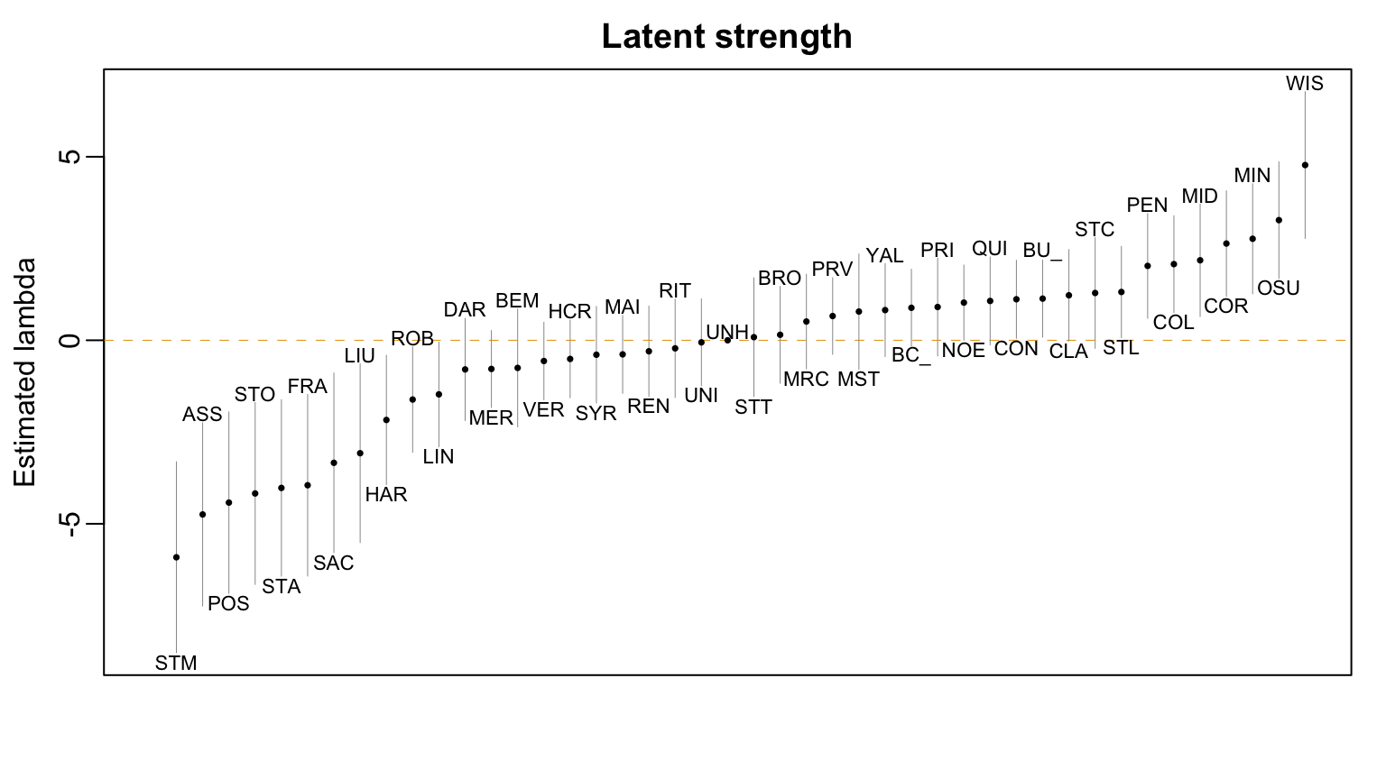
At WIS: 85.95 %

AT OSU: 76.67 %

AT neutral site: 81.76 %

Figure 1 shows the estimated latent strengths of all teams along with approximate 95% confidence intervals. The high degree of overlap between these marginal intervals suggests that there may be considerable uncertainty in the relative rankings of some teams. Precisely quantifying this uncertainty in rankings (e.g., with the bootstrap) is left as an Exercise.

Frozen 4 Simulation

Wisconsin, Ohio State, Cornell, and Minnesota qualified for the semi-finals of the 2025 NCAA Tournament (known as the Frozen 4). The teams were seeded as: (1) Wisconsin; (2) Ohio State; (3) Cornell; and (4) Minnesota. Following a standard bracket construction, the first semi-final game (which we will label SF1) was played between the 1st and 4th seed (Wisconsin vs Minnesota) and the second semi-final game (which we will label SF2) was played between the 2nd and 3rd seed (Ohio State vs Cornell).

Simulating the Original Tournament

To power our simulation, we will first enumerate all possible matchups between the four teams and compute the probability that the higher-seeded team wins. In computing these probabilities, we will account for the fact that all games were played at Ridder Arena, which is the home arena of Minnesota.

In the following code block, we first create a table containing the team names and their seeds. Then, we enumerate all possible combinations of teams using expand.grid().

seeds <- data.frame(
  Team = c("Wisconsin", "Ohio State", "Cornell", "Minnesota"),
  Seed = 1:4)

possible_matchups <-
  expand.grid(Hi = seeds$Team, Lo = seeds$Team) |>
  as.data.frame() |>
  dplyr::inner_join(y = seeds |> dplyr::rename(Hi = Team, Hi.Seed=Seed), by = "Hi") |>
  dplyr::inner_join(y = seeds |> dplyr::rename(Lo = Team, Lo.Seed=Seed), by = "Lo") |>
  dplyr::filter(Hi.Seed < Lo.Seed) |>
  dplyr::mutate(neutral = ifelse(Hi == "Minnesota" | Lo == "Minnesota", 0, 1)) |>
  dplyr::mutate(
    diff = lambda_hat[Hi, "ability"] - lambda_hat[Lo, "ability"],
    prob = dplyr::case_when(
      neutral == 1 ~ 1/(1 + exp(-1 * diff)),
      neutral == 0 & Hi == "Minnesota" ~ 1/(1 + exp(-1 * (diff + lambda0_hat))),
      neutral == 0 & Lo == "Minnesota" ~ 1/(1 + exp(-1 * (diff - lambda0_hat)))))

semis <- 
  data.frame(Hi = c("Wisconsin", "Ohio State"), Lo = c("Minnesota", "Cornell")) |>
  dplyr::left_join(possible_matchups |> dplyr::select(Hi, Lo, prob), by = c("Hi", "Lo"))

set.seed(479)
sf_winners <- c(NA, NA)

sf_outcomes <- rbinom(n = nrow(semis), size = 1, prob = semis$prob)
for(i in 1:nrow(semis)){
  if(sf_outcomes[i] == 1) sf_winners[i] <- semis$Hi[i]
  else sf_winners[i] <- semis$Lo[i]
}
cat("Semi-final outcomes:", sf_outcomes, "\n")
cat("Semi-final winners:", sf_winners, "\n")

1: The \(i\)-th entry of sf_outcomes is 1 if the higher-seed in game \(i\) wins and 0 if the lower-seed in game \(i\) wins

Semi-final outcomes: 0 1 
Semi-final winners: Minnesota Ohio State

The winners of both semi-final matches play each other in the finals. In the code below, we create a data frame containing the team names and then determine which is the higher seed. We then join the corresponding probability of the higher-seeded team winning the game. Finally, we simulate the outcome of the match and record the winner.

finals <- 
  data.frame(Team1 = sf_winners[1], Team2 = sf_winners[2]) |>
  dplyr::left_join(y = seeds |> dplyr::rename(Team1 = Team, Team1.Seed = Seed), by = "Team1") |>
  dplyr::left_join(y = seeds |> dplyr::rename(Team2 = Team, Team2.Seed = Seed), by = "Team2") |>
  dplyr::mutate(
    Hi = ifelse(Team1.Seed < Team2.Seed, Team1, Team2),
    Lo = ifelse(Team1.Seed < Team2.Seed, Team2, Team1)) |>
  dplyr::select(Hi, Lo) |> 
  dplyr::left_join(
    y = possible_matchups |> dplyr::select(Hi, Lo, prob), by = c("Hi", "Lo"))

final_outcome <- rbinom(n = 1, size = 1, prob = finals$prob)
if(final_outcome == 1){
  final_winner <- finals$Hi[1]
} else{
  final_winner <- finals$Lo[1]
}

cat("Finals outcome:", final_outcome, "\n")

Finals outcome: 1

cat("Finals winner:", final_winner, "\n")

Finals winner: Ohio State

In this simulation, Minnesota upset Wisconsin the first semi-finals; Ohio State beat Cornell in the second semi-finals; and Ohio State defeated Minnesota in the finals. Of course, if we run the simulation again with a different randomization seed, we might observe a different result. The code below runs simulates the Frozen 4 10,000 times. In each simulation iteration, we will save the winners of the two semi-final games (SF1_winner and SF2_winner); the two teams playing in the finals (Finals_Hi for the higher-seeded team and Finals_Lo for the lower-seeded team); and the eventual champion (Champion). By saving all these results, we can estimate the probabilities of not only simple events (e.g. \(\mathbb{P}(\textrm{Wisconsin wins the finals})\)) but also joint probabilities like \[\mathbb{P}(\textrm{Wisconsin makes it to and wins the finals})\] and conditional probabilities like \[ \mathbb{P}(\textrm{Wisconsin wins the finals} \vert \textrm{Wisconsin makes it to the finals}). \] by dividing the number of simulations in which Wisconsin wins the championship by beating Ohio State in the finals by the number of simulations in which Wisconsin plays Ohio State in the finals.

n_sims <- 10000

results <- data.frame(
  SF1_Winner = rep(NA, times = n_sims),
  SF2_Winner = rep(NA, times = n_sims),
  Finals_Hi = rep(NA, times = n_sims),
  Finals_Lo = rep(NA, times = n_sims),
  Champion = rep(NA, times = n_sims))


for(r in 1:n_sims){
  set.seed(479+r)
  sf_winners <- c(NA, NA)
  sf_outcomes <- rbinom(n = nrow(semis), size = 1, prob = semis$prob)
  for(i in 1:nrow(semis)){
    if(sf_outcomes[i] == 1){
      sf_winners[i] <- semis$Hi[i]
    } else{
      sf_winners[i] <- semis$Lo[i]
    }
    results[r, c("SF1_Winner", "SF2_Winner")] <- sf_winners
  }
  
  finals <- 
    data.frame(Team1 = sf_winners[1], Team2 = sf_winners[2]) |>
    dplyr::left_join(
      y = seeds |> dplyr::rename(Team1 = Team, Team1.Seed = Seed), 
      by = "Team1") |>
    dplyr::left_join(
      y = seeds |> dplyr::rename(Team2 = Team, Team2.Seed = Seed), 
      by = "Team2") |>
    dplyr::mutate(
      Hi = ifelse(Team1.Seed < Team2.Seed, Team1, Team2),
      Lo = ifelse(Team1.Seed < Team2.Seed, Team2, Team1)) |>
    dplyr::select(Hi, Lo) |> 
    dplyr::left_join(
      y = possible_matchups |> dplyr::select(Hi, Lo, prob), 
      by = c("Hi", "Lo"))
  
  results[r, "Finals_Hi"] <- finals$Hi[1]
  results[r, "Finals_Lo"] <- finals$Lo[1]
  
  final_outcome <- rbinom(n = 1, size = 1, prob = finals$prob)
  
  if(final_outcome == 1){
    results[r, "Champion"] <- finals$Hi[1]
  } else{
    results[r, "Champion"] <- finals$Lo[1]
  }
}

1: Data frame to hold the simulation results
2: Manually setting our randomization seed ensures reproducibility. But we need to use a different seed in every simulation iteration. Otherwise, we will get identical results across replications and that can bias our final probability estimates.
3: Save the winners of the semi-finals
4: Save the high and low seeds of the finals

Looking at the first several rows in results, we find that Wisconsin won the championship in most of the simulations.

results |> dplyr::slice_head(n = 10)

   SF1_Winner SF2_Winner  Finals_Hi  Finals_Lo   Champion
1   Wisconsin Ohio State  Wisconsin Ohio State  Wisconsin
2   Wisconsin Ohio State  Wisconsin Ohio State Ohio State
3   Wisconsin    Cornell  Wisconsin    Cornell  Wisconsin
4   Wisconsin Ohio State  Wisconsin Ohio State  Wisconsin
5   Wisconsin    Cornell  Wisconsin    Cornell  Wisconsin
6   Wisconsin Ohio State  Wisconsin Ohio State  Wisconsin
7   Wisconsin Ohio State  Wisconsin Ohio State  Wisconsin
8   Wisconsin Ohio State  Wisconsin Ohio State  Wisconsin
9   Wisconsin    Cornell  Wisconsin    Cornell  Wisconsin
10  Minnesota Ohio State Ohio State  Minnesota  Minnesota

In total, we find that Wisconsin won the championship in 7189 of the 10,000 simulation runs.

table(results$Champion)


   Cornell  Minnesota Ohio State  Wisconsin 
       502        765       1544       7189

Across the 10,000 simulations, we find that

Wisconsin made the finals in 8496 simulations
Wisconsin made and won the finals in 7189 simulations

Based on these numbers, we conclude that the conditional probability of Wisconsin winning the finals given that it made it to the finals is about 84.6%

sum(results$SF1_Winner == "Wisconsin" & results$Champion == "Wisconsin")/sum(results$SF1_Winner == "Wisconsin")

[1] 0.8461629

Simulating an Alternative Tournament

What if, instead of playing the semi-finals and finals at Ridder Arena, each game was held at the home arena of the higher-seeded team? Intuitively, we might expect Wisconsin’s chances of winning the championship to be much higher if they played all their matches at La Bahn Arena. To verify this, we will re-run our simulation. The only change is in the individual matchup probabilities: whereas in our original simulation, we only added the home advantage for Minnesota’s games, in our new simulation, we will add the advantage to all games.

alt_matchups <-
  expand.grid(Hi = seeds$Team, Lo = seeds$Team) |>
  as.data.frame() |>
  dplyr::inner_join(y = seeds |> dplyr::rename(Hi = Team, Hi.Seed=Seed), by = "Hi") |>
  dplyr::inner_join(y = seeds |> dplyr::rename(Lo = Team, Lo.Seed=Seed), by = "Lo") |>
  dplyr::filter(Hi.Seed < Lo.Seed) |>
  dplyr::mutate(
    diff = lambda_hat[Hi, "ability"] - lambda_hat[Lo, "ability"],
    log_odds = diff + lambda0_hat,
    prob = 1/(1 + exp(-1 * (log_odds))))

semis <- 
  data.frame(Hi = c("Wisconsin", "Ohio State"), Lo = c("Minnesota", "Cornell")) |>
  dplyr::left_join(alt_matchups |> dplyr::select(Hi, Lo, prob), by = c("Hi", "Lo"))

1: This is the log-odds of the higher seed winning if the game were played at a neutral site
2: In this alternative, the higher seed always plays at a home, hence the additional lambda0_hat factor.
3: Recreate semis but include the new matchup probabilities for the alternative scenario

n_sims <- 10000

alt_results <- data.frame(
  SF1_Winner = rep(NA, times = n_sims),
  SF2_Winner = rep(NA, times = n_sims),
  Finals_Hi = rep(NA, times = n_sims),
  Finals_Lo = rep(NA, times = n_sims),
  Champion = rep(NA, times = n_sims))

for(r in 1:n_sims){
  set.seed(479+r)
  sf_winners <- c(NA, NA)
  sf_outcomes <- rbinom(n = nrow(semis), size = 1, prob = semis$prob)
  for(i in 1:nrow(semis)){
    if(sf_outcomes[i] == 1){
      sf_winners[i] <- semis$Hi[i]
    } else{
      sf_winners[i] <- semis$Lo[i]
    }
    alt_results[r, c("SF1_Winner", "SF2_Winner")] <- sf_winners
  }
  
  finals <- 
    data.frame(Team1 = sf_winners[1], Team2 = sf_winners[2]) |>
    dplyr::left_join(
      y = seeds |> dplyr::rename(Team1 = Team, Team1.Seed = Seed), 
      by = "Team1") |>
    dplyr::left_join(
      y = seeds |> dplyr::rename(Team2 = Team, Team2.Seed = Seed), 
      by = "Team2") |>
    dplyr::mutate(
      Hi = ifelse(Team1.Seed < Team2.Seed, Team1, Team2),
      Lo = ifelse(Team1.Seed < Team2.Seed, Team2, Team1)) |>
    dplyr::select(Hi, Lo) |> 
    dplyr::left_join(
      y = possible_matchups |> dplyr::select(Hi, Lo, prob), 
      by = c("Hi", "Lo"))
  
  alt_results[r, "Finals_Hi"] <- finals$Hi[1]
  alt_results[r, "Finals_Lo"] <- finals$Lo[1]
  
  final_outcome <- rbinom(n = 1, size = 1, prob = finals$prob)
  
  if(final_outcome == 1){
    alt_results[r, "Champion"] <- finals$Hi[1]
  } else{
    alt_results[r, "Champion"] <- finals$Lo[1]
  }
}

In the alternative competition, where the higher-seeded team plays at home, we estimate that Wisconsin would win the championship about 77% of the time, up from the 71% in the version of the tournament played a neutral site.

table(alt_results$Champion)


   Cornell  Minnesota Ohio State  Wisconsin 
       360        418       1533       7689

Exercises

Use the bootstrap to quantify the uncertainty in relative rankings of each team. To do this, you will need to re-sample individual games, re-compute the numbers of home & away team wins for every combination of teams and neutral, and fit a Bradley-Terry model. Report the number of bootstrap simulations in which Wisconsin was ranked 1st and also report a 95% bootstrap confidence interval for Wisconsin’s overall rank.
Build a simulation for the entire NCAA Tournament based on the estimating probabilities from our Bradley-Terry model that accounts for home advantage. In this tournament, the first round and quarterfinals were held on the campuses of the top-4 seeded teams (Wisconsin, Ohio State, Cornell, and Minnesota). Subsequent games were played at Ridder Arena at the University of Minnesota. Your simulation should involve only the 11 teams who actually played in the tournament

Footnotes

Remember, this is restriction is needed because the \(\lambda_{j}\)’s are otherwise not identifiable. Without this restriction, the data gives us know way to distinguish between one set of values for the \(\lambda_{j}\)’s and another set that shifts all the values by the same fixed constant. See Lecture 12 for more details.↩︎
R implements data frames using a list data type, with each column representing a separate list element. So, what we’re really doing here is adding a list-valued element to a list, which is easier to interpret than a data frame-valued column in a data frame.↩︎