Lecture 6: Run Expectancy

Motivation: Credit Allocation in Baseball

The first game of the 2024 MLB Regular Season, between the Los Angeles Dodgers and the San Diego Padres, took place on March 20, 2024¹ During the game, Shohei Ohtani recorded two hits in his five plate appearances:

In the 3rd inning, with 2 outs and no runners on base, Ohtani singled into right field.
In the 8th inning, with 1 out and runners on first and second base, Ohtani singled into left center field, driving in one run.

Which of these singles was more valuable to Dodgers? And how much of that value should be specifically credited to Ohtani?

Because the second single directly resulted in a run scoring, it is tempting to conclude that the second single was more valuable than the first. However, although the Dodgers didn’t score as a result of the first single, Ohtani reached first base, putting his team in a position to potential score more runs than if he had not reached first². In terms of allocating credit, it seems natural to give Ohtani all the credit for whatever value was created on his first single. But on his second single, at least some of the value created is attributable to a baserunner scoring from second base. How should we divide credit between Ohtani and that baserunner?

Over the next several lectures, we will work with pitch-level tracking data from Major League Baseball to answer these questions. In this lecture, we begin by computing the number of runs that a team can expect to score in the remainder of a half-inning (Section 4). Then, we introduce run values (Section 5), a metric that combines changes in the number of a team expects to score and the number of runs actually scored in an at-bat. We conclude by determining which batters created the most run value for their teams (Section 6).

In Lecture 7, we will distribute the run value created in every at-bat between the batter and base runners involved in the at-bat. We will then begin Lecture 8 by distributing the negative of the run value created by th batting team between the pitcher and fielders involved in each at-bat. Finally, we will aggregate the total run value over average created by each player through their hitting, fielding, base running, and pitching and convert that aggregate into a measure of wins above replacement. Our development largely follows (Baumer, Jensen, and Matthews 2015), who created a transparent, open-source version of wins above replacement, a cornerstone of baseball analytics.

Tracking Data in Baseball

A Brief History

On October 4, 2006, during an American League Division Series game between the Oakland Athletics and Minnesota Twins, the sports media company Sportvision³ debuted PitchF/X⁴, a system of cameras for tracking the position of every pitch as it traveled from the pitcher’s hand to the batter. After installing the system in every MLB ballpark, Sportvision began providing the data in real-time data to the MLB. These data, combined with additional information recorded by an MLB Advanced Media employee, powered the popular GameDay application and were publicly available through the GameDay application programming interface (API) for many years.

In 2017, PITCHf/x system was phased out replaced by the radar-based Trackman system, which was originally developed to track the trajectories of golf balls. Trackman is part of the larger Statcast system, which additionally tracks the movement of all players on the field. See this New York Times article for more about the history of Statcast.

Accessing Statcast Data in R

Major League Baseball hosts a public-facing web interface for accessing Statcast data. Using that interface, users can pull up data for individual players or about all pitches of a certain type. Powering this website is an API, which allows software applications to connect to the underlying Statcast database. It is through this API that the baseballr package acquires data. You can install the package with the code:

devtools::install_github(repo = "BillPetti/baseballr")

The function baseballr::statcast_search() allows users query all Statcast data by date, player, or player type. One of the original baseballr authors, Bill Petti, wrote a wrapper function that uses baseballr::statcast_search() to pull down an entire season’s worth of pitch-by-pitch data; see this blog post for the wrapper function code and this earlier post for details about its design. Since he published his original function, Statcast has added some new fields, necessitating a few changes to the original script. The code below defines a new scraper, which we will use in the course. An R script containing this code is available at this link. At a high level, the scraping function pulls data from Statcast on a week-by-week basis.

Show the code for Statcast scraper

## Code modified from Bill Petti's original annual Statcast scraper:
## Main change is in the column names of the fielders

annual_statcast_query <- function(season) {
  
  data_base_column_types <- 
    readr::read_csv("https://app.box.com/shared/static/q326nuker938n2nduy81au67s2pf9a3j.csv")
  
  dates <- 
    seq.Date(as.Date(paste0(season, '-03-01')),
             as.Date(paste0(season, '-12-01')), 
             by = '4 days')
  
  date_grid <- 
    tibble::tibble(start_date = dates, 
                   end_date = dates + 3)
  
  safe_savant <- 
    purrr::safely(baseballr::scrape_statcast_savant)
  
  payload <- 
    purrr::map(.x = seq_along(date_grid$start_date),
               ~{message(paste0('\nScraping week of ', date_grid$start_date[.x], '...\n'))
                 payload <- 
                   safe_savant(start_date = date_grid$start_date[.x], 
                               end_date = date_grid$end_date[.x], 
                               type = 'pitcher')
                 return(payload)
               })
  
  payload_df <- purrr::map(payload, 'result')
  
  number_rows <- 
    purrr::map_df(.x = seq_along(payload_df),
                  ~{number_rows <- 
                    tibble::tibble(week = .x, 
                                   number_rows = length(payload_df[[.x]]$game_date))
                  }) %>%
    dplyr::filter(number_rows > 0) %>%
    dplyr::pull(week)
  
  payload_df_reduced <- payload_df[number_rows]
  
  payload_df_reduced_formatted <- 
    purrr::map(.x = seq_along(payload_df_reduced), 
               ~{cols_to_transform <- 
                 c("pitcher", "fielder_2", "fielder_3",
                   "fielder_4", "fielder_5", "fielder_6", "fielder_7",
                   "fielder_8", "fielder_9")
               df <- 
                 purrr::pluck(payload_df_reduced, .x) %>%
                 dplyr::mutate_at(.vars = cols_to_transform, as.numeric) %>%
                 dplyr::mutate_at(.vars = cols_to_transform, function(x) {ifelse(is.na(x), 999999999, x)})
               character_columns <- 
                 data_base_column_types %>%
                 dplyr::filter(class == "character") %>%
                 dplyr::pull(variable)
               numeric_columns <- 
                 data_base_column_types %>%
                 dplyr::filter(class == "numeric") %>%
                 dplyr::pull(variable)
               integer_columns <- 
                 data_base_column_types %>%
                 dplyr::filter(class == "integer") %>%
                 dplyr::pull(variable)
               df <- 
                 df %>%
                 dplyr::mutate_if(names(df) %in% character_columns, as.character) %>%
                 dplyr::mutate_if(names(df) %in% numeric_columns, as.numeric) %>%
                 dplyr::mutate_if(names(df) %in% integer_columns, as.integer)
               return(df)
               })
  
  combined <- payload_df_reduced_formatted %>%
    dplyr::bind_rows()
  
  return(combined)
}

To use this function, it is enough to run something like.

raw_statcast2024 <- annual_statcast_query(2024)

Warning

Scraping a single season of Statcast data can take between 30 and 45 minutes. I highly recommend scraping the data for any season only once and saving the resulting data table in an .RData file that can be loaded into future R sessions.

library(tidyverse)
raw_statcast2024 <- annual_statcast_query(2024)
save(raw_statcast2024, file = "raw_statcast2024.RData")

These .RData files take between 75MB and 150MB of space. So, if you want to work with data from all available seasons (2008 to the present), you will need about 2.5GB of storage space on your computer.

Statcast Basics

The function annual_statcast_query actually scrapes data not only from the regular season but also from the pre-season and the play-offs. The column game_type records the type of game in which each pitch was thrown. Looking at the Statcast documentation, we see that regular season pitches have game_type=="R".

table(raw_statcast2024$game_type, useNA = 'always')


     D      F      L      R      S      W   <NA> 
  5182   2488   3540 695136  77056   1576      0

For our analyses, we will work only with data from regular season games. Below, we filter to those pitches with game_type=="R" and remove those with non-sensical values like 4 balls or 3 strikes.

statcast2024 <-
  raw_statcast2024 |> 
  dplyr::filter(game_type == "R") |>
  dplyr::filter(
    strikes >= 0 & strikes < 3 & 
      balls >= 0 & balls < 4 & 
      outs_when_up >= 0 & outs_when_up < 3) |>
  dplyr::arrange(game_date, game_pk, at_bat_number, pitch_number)

We’re now left with 695,135 regular season pitches.

Pitch- and At-Bat-level Descriptions

Statcast records a ton of information about each pitch including the type of pitch (pitch_type), the velocity of the pitch when it was released (vx0, vy0, vz0), the acceleration of the pitch at about the half-way point between the pitcher and batter (ax, ay, and az), and horizontal and vertical coordinates of the pitch as it crosses the front edge of home plate (plate_x) and (plate_y). The column type also records whether the pitch resulted ball (type=B), a strike (type=S), or whether the ball was put in play (type=X). For balls in play, Statcast also records things like the launch speed and angle (launch_speed, launch_angle), the coordinates on the field where the ball landed (hc_x) and (hc_y), and the position of the first fielder to touch the ball (hit_location). In Lecture 8, we will work with hc_x and hc_y to build a model that predicts the probability that each fielder makes an out on balls hit to a specific part of the field. As a bit of a preview, here is a plot of all the hc_x and hc_y values.

par(mar = c(3,3,2,1), mgp = c(1.8, 0.5, 0))
plot(statcast2024$hc_x, statcast2024$hc_y, 
     xlab = "hc_x", ylab = "hc_y",
     pch = 16, cex = 0.2, col = rgb(0,0,0, 0.1))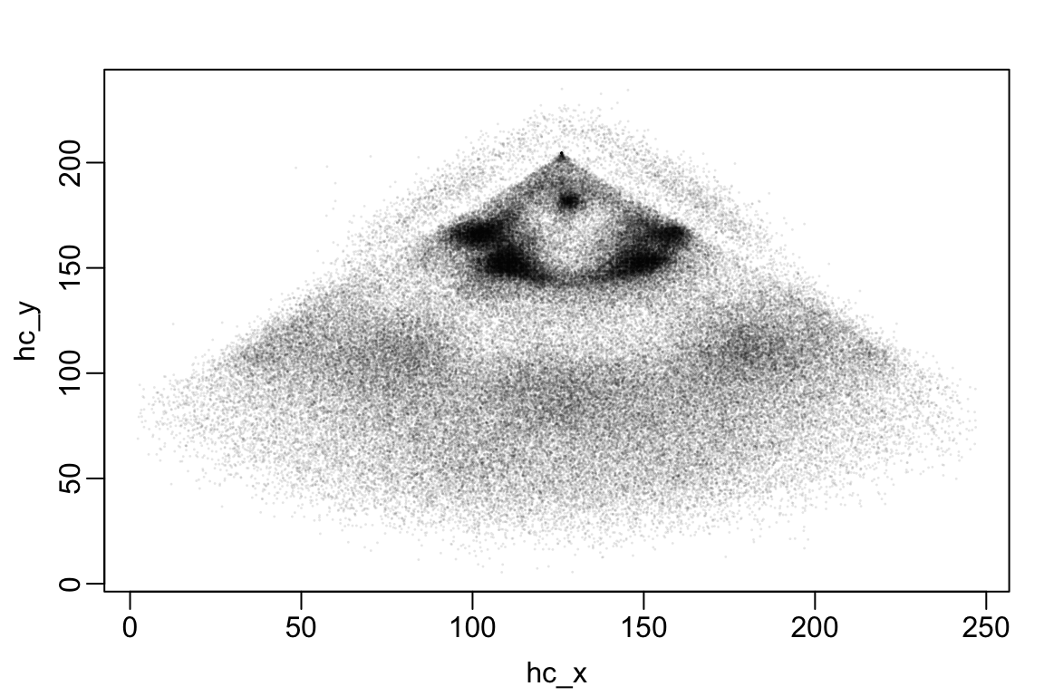

Adding Baserunner Information

The columns on_1b, on_2b, and on_3b record who is on first, second, or third base at the beginning of each pitch (NA values indicate that nobody is on base). For convenience, we will add a new column to the data table that records the baserunner configuration using a string of 3 binary digits. If there is a runner on first base, the first digit will be a 1 and if there is not a runner on first base, the first digit will be a 0. Similarly, the second and third digits respectively indicate whether there are runners on second and third base. So, the string "101" indicates that there are runners on first and third base but not on second. To create the 3-digit binary string encoding baserunner configuration, notice that 1*(!is.na(on_1b)) will return a 1 if there is someone on first base and 0 otherwise. So by pasting together the results of 1*(!is.na(on_1b)), 1*(!is.na(on_2b)), and 1*(!is.na(on_3b)), we can form the 3-digit binary string described above. In following code, we also rename the column outs_when_up to Outs.

statcast2024 <-
  statcast2024 |>
  dplyr::mutate(
    BaseRunner = 
      paste0(1*(!is.na(on_1b)),1*(!is.na(on_2b)),1*(!is.na(on_3b)))) |>
  dplyr::rename(Outs = outs_when_up)

Getting Player Names

For every pitch, the Statcast dataset records the identities of the batter (batter), pitcher (pitcher), and the other fielders (fielders_2, …, fielders_9). However, it does not identify them by name, instead using an ID number, which is assigned by MLB Advanced Media. We can look up the corresponding player names using a database maintained by the Chadwick Register. The function baseballr::chadwick_player_lu() downloads the Chadwick database and stores it as a data table in R. This database contains the names and MLB Advanced Media identifiers for players across all seasons, far more than we need for our purposes. So, in the code below, we first download the Chadwick player database and then extract only those players who appeared in the 2024 regular season. Like with the raw pitch-by-pitch data, I recommend that you download this player identity database once and save the table as an .RData object for future use.

player2024_id <-
  unique(
    c(statcast2024$batter, statcast2024$pitcher,
      statcast2024$on_1b, statcast2024$on_2b, statcast2024$on_3b,
      statcast2024$fielder_2, statcast2024$fielder_3,
      statcast2024$fielder_3, statcast2024$fielder_4,
      statcast2024$fielder_5, statcast2024$fielder_6,
      statcast2024$fielder_7, statcast2024$fielder_8,
      statcast2024$fielder_9))

chadwick_players <- baseballr::chadwick_player_lu()
save(chadwick_players, file = "chadwick_players.RData")

player2024_lookup <-
  chadwick_players |>
  dplyr::filter(!is.na(key_mlbam) & key_mlbam %in% player2024_id) |>
  dplyr::mutate(
    FullName = paste(name_first, name_last),
    Name = stringi::stri_trans_general(FullName, "Latin-ASCII"))
save(player2024_lookup, file = "player2024_lookup.RData")

1: This vector contains the MLB Advanced Media ID for all players who appeared in 2024 as a batter, pitcher, fielder, or baserunner.
2: Save a local copy of the full Chadwick database.
3: Creates a column containing the player’s first and last name.
4: Removes any accents or special characters, which we will need in Lecture 7.

Getting Player Positions

Later in Lecture 7, we will compare each batter’s hitting performance to the average performance of other batters who play the same position in the field. Unfortunately, the Chadwick database does not record the position of each player. Luckily, position information can be obtained using baseballr::mlb_batting_orders(), which retrieves the batting order for each MLB game. In this functions output, the column id contains the MLB Advanced Media id number for each player (i.e., key_mlbam in the data table player2024_lookup that we created above) and the column abbreviation contains the fielding position. For instance, Ohtani was listed as the Designated Hitter in that March 20, 2024 game between the Dodgers and the Padres.

baseballr::mlb_batting_orders(game_pk = 745444)

── MLB Game Starting Batting Order data from MLB.com ─── baseballr 1.6.0.9002 ──

ℹ Data updated: 2025-08-19 18:11:54 CDT

# A tibble: 18 × 8
       id fullName         abbreviation batting_order batting_position_num team 
    <int> <chr>            <chr>        <chr>         <chr>                <chr>
 1 605141 Mookie Betts     SS           1             0                    away 
 2 660271 Shohei Ohtani    DH           2             0                    away 
 3 518692 Freddie Freeman  1B           3             0                    away 
 4 669257 Will Smith       C            4             0                    away 
 5 571970 Max Muncy        3B           5             0                    away 
 6 606192 Teoscar Hernánd… RF           6             0                    away 
 7 681546 James Outman     CF           7             0                    away 
 8 518792 Jason Heyward    RF           8             0                    away 
 9 666158 Gavin Lux        2B           9             0                    away 
10 593428 Xander Bogaerts  2B           1             0                    home 
11 665487 Fernando Tatis … RF           2             0                    home 
12 630105 Jake Cronenworth 1B           3             0                    home 
13 592518 Manny Machado    DH           4             0                    home 
14 673490 Ha-Seong Kim     SS           5             0                    home 
15 595777 Jurickson Profar LF           6             0                    home 
16 669134 Luis Campusano   C            7             0                    home 
17 642180 Tyler Wade       3B           8             0                    home 
18 701538 Jackson Merrill  CF           9             0                    home 
# ℹ 2 more variables: teamName <chr>, teamID <int>

Because baseballr::mlb_batting_orders() can be run using only one game identifier (i.e., game_pk) at a time, we need to loop over all of the unique game_pk values in statcast2024 to get all batting orders. In the code block below, we first create a wrapper function, which we call get_lineup around baseballr::mlb_batting_orders() that only retains the columns id and abbreviation and renames those columns.

get_lineup <- function(game_pk){
  lineup <- baseballr::mlb_batting_orders(game_pk = game_pk)
  lineup <-
    lineup |>
    dplyr::mutate(game_pk = game_pk) |>
    dplyr::rename(key_mlbam = id, position = abbreviation) |>
    dplyr::select(game_pk, key_mlbam, position)
  return(lineup)
}

Now, to get the batting orders for all regular season games from 2024, we could try writing a for loop that iterates over all unique game_pk values and writes the table to a list.

all_lineups <- list()
unik_game_pk <- unique(statcast2024$game_pk)
for(i in 1:length(unik_game_pk)){
  all_lineups[[i]] <- get_lineup(game_pk = unik_game_pk[i])
}

If get_lineup() throws an error (e.g., because the batting orders for a particular game are not available), then the whole loop gets terminated. To avoid having to manually remove problematic games and re-start the loop, we will use purrr:possibly() to create a version of get_lineup() that returns NULL when it hits an error. We will also use purrr:map instead of writing an explict for loop.

Warning

The following code takes about an hour to run.

poss_get_lineup <- purrr::possibly(.f = get_lineup, otherwise = NULL) 
unik_game_pk <- unique(statcast2024$game_pk)

block_starts <- seq(1, length(unik_game_pk), by = 500)
block_ends <- c(block_starts[-1], length(unik_game_pk))

all_lineups <- list()
for(b in 1:5){
  tmp <-
    purrr::map(.x = unik_game_pk[block_starts[b]:block_ends[b]], 
               .f = poss_get_lineup, 
               .progress = TRUE)
  all_lineups <- c(all_lineups, tmp)
}

lineups2024 <- 
  dplyr::bind_rows(all_lineups) |>
  unique()
save(lineups2024, file = "lineups2024.RData")

1: I was not able to loop over the whole set of unique game_pk values at once. I found it useful to break the loop into blocks of about 500 games each.
2: Each element of all_lineup is a data table. This allows us to stack them on top of one another.
3: It’s useful to save the table of batting orders just in case we need it again in the future

The table lineups2024 contains the starters and their position for all the games in our dataset. The following code determines the most commonly listed position for each player.

positions2024 <-
  lineups2024 |>
  dplyr::group_by(key_mlbam, position) |>
  dplyr::summarise(n = dplyr::n()) |>
  dplyr::slice_max(order_by = n, with_ties = FALSE) |>
  dplyr::ungroup() |>
  dplyr::select(key_mlbam, position)
save(positions2024, file = "positions2024.RData")

1: Counts the number of occurrences of each player-position combination
2: After we call dplyr::summarise(), the resulting data table is still grouped by batter. So, when we call dplyr::slice_max() it looks at all the rows corresponding to each player and extracts the one with highest count. This is how we determine the most commonly listed position.

Expected Runs

Definition: Expected Runs

For each combination of the number of outs (\(\textrm{o} \in \{0,1,2\}\)) and base runner configurations (\(\textrm{br} \in \{"000", "100", "010", "001", "110", "101", "011", "111"\}\)), let \(\rho(\textrm{o}, \textrm{br})\) be the average number of runs that a team scores in the remainder of the half-inning following a pitch thrown with \(\textrm{o}\) outs and base runner configuration \(\textrm{br}.\)

Computing \(\rho(\textrm{o}, \textrm{br})\) is conceptually straightforward: we need to divide our observed at-bats into 24 bins, one for each combination of \((\textrm{o}, \textrm{br})\) and then compute the average value of \(R\) within each bin. This is exactly the same “binning-and-averaging” procedure we used to fit our initial XG models in Lecture 2. We will do this using pitches taken in the first 8 innings of played in the 2024 regular season. We focus only on the first 8 innings because the 9th and extra innings are fundamentally different than the others. Specifically, the bottom half of the 9th (or later) innings is only played if the game is tied or the home team is trailing after the top of the 9th inning concludes. In those half-innings, if played, the game stops as soon as a winning run is scored. For instance, say that the home team is trailing by 1 runs in the bottom of the 9th and that there are runners on first and second base. If the batter hits a home run, the at-bat is recorded as resulting in only two runs (the tying run from second and the winning run from first). But the exact same scenario would result in 3 runs in an earlier inning.

Computing Runs Scored in the Half-Inning

Suppose that in a given at-bat \(a\) that there are \(n_{a}\) pitches. Within at-bat \(a,\) for each \(i = 1, \ldots, n_{a},\) let \(R_{i,a}\) be the number of runs scored in the half-inning after that pitch (including any runs scored as a result of pitch \(i\)). So \(R_{1,a}\) is the number of runs scored in the half-inning after the first pitch, \(R_{2,a}\) is the number of runs scored subsequent to the second pitch, etc. Our first step towards building the necessary at-bat-level data set will be to append a column of \(R_{i,a}\) values to each season’s Statcast data.

We start by illustrating the computation using a single half-inning from the Dodgers-Padres game introduced earlier. The code below pulls out all pitches thrown in the top of the 8th inning of the game. During this inning, the Dodgers scored 4 runs.

dodgers_inning <-
  statcast2024 |>
  dplyr::filter(game_pk == 745444 & inning == 8 & inning_topbot == "Top") |>
  dplyr::select(
    at_bat_number, pitch_number, Outs, BaseRunner,
    bat_score, post_bat_score, events, description, des,
    type, on_1b, on_2b, on_3b, hc_x, hc_y, hit_location) |>
  dplyr::arrange(at_bat_number, pitch_number)

The column bat_score records the batting team’s score before each pitch is thrown. The column post_bat_score records the batting team’s score after the the outcome of the pitch. For most of the 25 pitches, we find that bat_score is equal to post_bat_score; this is because only a few pitches result in scoring events.

rbind(bat_score = dodgers_inning$bat_score, post_bat_score = dodgers_inning$post_bat_score)

               [,1] [,2] [,3] [,4] [,5] [,6] [,7] [,8] [,9] [,10] [,11] [,12]
bat_score         1    1    1    1    1    1    1    1    1     1     1     1
post_bat_score    1    1    1    1    1    1    1    1    1     1     1     1
               [,13] [,14] [,15] [,16] [,17] [,18] [,19] [,20] [,21] [,22]
bat_score          1     1     2     3     3     3     4     5     5     5
post_bat_score     1     2     3     3     3     4     5     5     5     5
               [,23] [,24] [,25]
bat_score          5     5     5
post_bat_score     5     5     5

Cross-referencing the table above with the play-by-play data, we see that the Dodgers score their second run after the 14th pitch of the half-inning (on a Enrique Hernández sacrifice fly); their third run on the very next pitch (Gavin Lux grounding into a fielder’s choice); and their fourth and fifth runs on consecutive pitches (on singles by Mookie Betts and Shohei Ohtani).

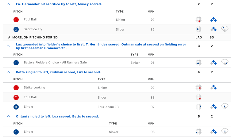
Figure 1: Play-by-Play from the March 20, 2024 Dodgers-Padres game

We can verify this by looking at the variable des, which stores a narrative description about what happened during the at-bat.

dodgers_inning$des[c(14,15, 18, 19)]

[1] "Enrique Hernández out on a sacrifice fly to left fielder José Azocar. Max Muncy scores."                                                                                             
[2] "Gavin Lux reaches on a fielder's choice, fielded by first baseman Jake Cronenworth. Teoscar Hernández scores. James Outman to 2nd. Fielding error by first baseman Jake Cronenworth."
[3] "Mookie Betts singles on a ground ball to left fielder José Azocar. James Outman scores. Gavin Lux to 2nd."                                                                           
[4] "Shohei Ohtani singles on a line drive to left fielder José Azocar. Gavin Lux scores. Mookie Betts to 2nd."

Notice that, because we’ve sorted the pitches in ascending order by at-bat and pitch number, the very last row of the table corresponds to the last pitch of the inning. Accordingly, the last value in the post_bat_score column is the batting team’s score at the end of the inning. Thus, to compute \(R_{i,a}\) for all pitches in this inning, it is enough to subtract the bat_score in each row from the last post_bat_score in the table. To access this last value, we use the function last().

dplyr::last(dodgers_inning$post_bat_score) - dodgers_inning$bat_score

 [1] 4 4 4 4 4 4 4 4 4 4 4 4 4 4 3 2 2 2 1 0 0 0 0 0 0

We now append a column with these values to our data table dodgers_inning

dodgers_inning <-
  dodgers_inning |>
  dplyr::mutate(RunsRemaining = dplyr::last(post_bat_score) - bat_score)

Putting It All Together

We’re now ready to extend these calculation to every half-inning of every game in the season. To do this, we will take advantage of the dplyr::group_by() function to apply the same calculation to subsets defined by game and half-inning.

statcast2024 <-
  statcast2024 |>
  dplyr::group_by(game_pk, inning, inning_topbot) |>
  dplyr::arrange(at_bat_number, pitch_number) |>
  dplyr::mutate(RunsRemaining = dplyr::last(post_bat_score) - bat_score) |>
  dplyr::ungroup()

1: Divide the data based on the combination of game and half-inning
2: Arrange pitches in the appropriate temporal order
3: Add column for how many runs were scored after each pitch

Now we have the number of runs scored in the half-inning after each pitch. But to compute run expectancy, we need this quantity at the at-bat level and not at the pitch-level. Using our notation from before, note that \(R_{1,a}\) is the number of runs scored after the first pitch of at-bat \(a.\) So, to compute run expectancy, it is enough to pull out the first pitch from each at-bat (i.e., those pitches with pitch_number == 1) using the filter() function.

expected_runs <-
  statcast2024 |>
  dplyr::filter(pitch_number == 1) |>
  dplyr::select(Outs, BaseRunner, RunsRemaining) |>
  dplyr::group_by(Outs, BaseRunner) |>
  dplyr::summarize(rho = mean(RunsRemaining), .groups = "drop")

1: Get the first pitch in every at-bat
2: Sub-divide the data based on the 24 combinations of out and baserunner
3: Compute the mean of RunRemaining for each game state combination

The table expected_runs contains one row for every combination of outs and base-runner configuration. Traditionally, expected runs is reported using an \(8\times 3\) matrix, with rows corresponding to base-runner configurations and columns corresponding to outs. We can re-format expected_runs to this matrix format using the tidyr::pivot_wider() function

expected_runs |> 
  tidyr::pivot_wider(
    names_from = Outs,
    values_from = rho,
    names_prefix="Outs: ")

# A tibble: 8 × 4
  BaseRunner `Outs: 0` `Outs: 1` `Outs: 2`
  <chr>          <dbl>     <dbl>     <dbl>
1 000            0.488     0.262    0.0980
2 001            1.43      0.972    0.352 
3 010            1.07      0.672    0.347 
4 011            2.03      1.44     0.612 
5 100            0.897     0.529    0.228 
6 101            1.90      1.22     0.502 
7 110            1.49      0.926    0.449 
8 111            2.31      1.58     0.815

In the March 20, 2024 game against the Padres, Ohtani recorded his first hit in the 3rd inning on a pitch with 2 outs and no runners on base. Based on the game state at the start of the at-bat (i.e., Outs=2 and BaseRunner='000'), his team can expect to score 0.1 runs in the remainder of the half-inning. As a result of Ohtani’s single, he changed the game state to Outs = 2 and BaseRunner=100, a state from which his team can expect to score 0.22 runs, on average. So, although his at-bat did not directly result in a run scoring, Ohtani increased his team’s run expectancy by about 0.12 runs.

Run Value

While expected runs is a really useful metric, for the purposes of allocating credit, we need to account not only for what we expect to happen but also what actually happened as a result of each at-bat.

Definition: Run Value

The run value of an at-bat is defined as the the number of runs scored in the at-bat plus the difference in expected runs from the starting to ending state. That is, denoting the number of runs scored in the at-bat as \(\textrm{RunsScored}\) and the starting and ending states as \((\textrm{o}_{\text{start}}, \textrm{br}_{\text{start}})\) and \((\textrm{o}_{\text{end}}, \textrm{br}_{\text{end}}),\) then \[ \textrm{RunValue} = \textrm{RunsScored} + \rho(\textrm{o}_{\text{end}}, \textrm{br}_{\text{end}}) - \rho(\textrm{o}_{\text{start}}, \textrm{br}_{\text{start}}) \]

In a sense, run value rewards batters and base runners for two things, actually scoring runs and putting their team in positions from which they could potentially score more runs.

Tocompute the run value of each at-bat in the 2024 season, we must compute

The number of runs scored during each at-bat
The game state (i.e., the number of outs and the base-runner configuration) at the start and end of each at-bat
The change in expected runs during the at-bat (i.e., \(\rho(\textrm{o}_{\text{end}}, \textrm{br}_{\text{end}}) - \rho(\textrm{o}_{\text{start}}, \textrm{br}_{\text{start}})\)).

We will first develop the necessary code using the data from Dodger’s 8th inning from their game against the Padres. Then, we will deploy that code to the whole statcast2024 table by grouping by game_pk and at_bat_number.

Calculating Runs Score

Statcast numbers every at-bat within the game and every pitch within each at-bat. To compute the number of runs scored within each at-bat, we will:

Sort the pitches by at-bat number and then by pitch number in ascending order
Take the difference between the last value of post_bat_score and first value of bat_score within each at-bat.

Let’s try to verify this by looking at pitches from the third, fourth, and fifth at-bats of Dodgers’ 8th inning against the Padres⁵

dodgers_inning |>
  dplyr::filter(at_bat_number %in% 61:63) |>
  dplyr::arrange(at_bat_number, pitch_number) |>
  dplyr::select(at_bat_number, pitch_number, bat_score, description, post_bat_score)

── MLB Baseball Savant Statcast Search data from baseballsavant.mlb.com ────────

ℹ Data updated: 2025-06-21 09:37:16 CDT

# A tibble: 7 × 5
  at_bat_number pitch_number bat_score description   post_bat_score
          <int>        <int>     <dbl> <chr>                  <dbl>
1            61            1         1 ball                       1
2            61            2         1 ball                       1
3            61            3         1 ball                       1
4            61            4         1 ball                       1
5            62            1         1 foul                       1
6            62            2         1 hit_into_play              2
7            63            1         2 hit_into_play              3

Based on the description column, we see that the first pitch of at-bat 62 was a foul ball and the second pitch was hit into play. When we look at the corresponding row (row 6) of the table, we see that that Dodgers’ pre-pitch score was 1 (bat_score = 1) and that they scored 1 run as a result of the hit (post_bat_score = 2). Reassuringly, the difference between the value of post_bat_score in row 6 (the last row for at-bat 62) and the value of bat_score in row 5 (the first row for at-bat 62) is 1. We can similarly verify our procedure works in at-bat 61: the fourth value of post_bat_score and the first value of bat_score are equal and the Dodgers did not score in this at-bat.

We can apply our procedure to the entirety of the Dodgers’ half-inning

dodgers_inning <-
  dodgers_inning |>
  dplyr::group_by(at_bat_number) |>
  dplyr::arrange(pitch_number) |>
  dplyr::mutate(RunsScored = dplyr::last(post_bat_score) - dplyr::first(bat_score)) |>
  dplyr::ungroup() |>
  dplyr::arrange(at_bat_number, pitch_number)
dodgers_inning |> dplyr::select(at_bat_number, pitch_number, bat_score, description, post_bat_score, RunsScored)

# A tibble: 25 × 6
   at_bat_number pitch_number bat_score description   post_bat_score RunsScored
           <int>        <int>     <dbl> <chr>                  <dbl>      <dbl>
 1            59            1         1 called_strike              1          0
 2            59            2         1 ball                       1          0
 3            59            3         1 ball                       1          0
 4            59            4         1 foul                       1          0
 5            59            6         1 blocked_ball               1          0
 6            60            1         1 ball                       1          0
 7            60            2         1 foul_tip                   1          0
 8            60            3         1 hit_into_play              1          0
 9            61            1         1 ball                       1          0
10            61            2         1 ball                       1          0
# ℹ 15 more rows

We can now apply this formula to all pitches in statcast2024 by grouping by game_pk and at_bat_number. We will also save a copy of the data table statcast2024 so that we can load it into future R sessions.

statcast2024 <-
  statcast2024 |>
  dplyr::group_by(game_pk, at_bat_number) |>
  dplyr::arrange(pitch_number) |>
  dplyr::mutate(RunsScored = dplyr::last(post_bat_score) - dplyr::first(bat_score)) |>
  dplyr::ungroup() |>
  dplyr::arrange(game_date, game_pk, at_bat_number, pitch_number)

save(statcast2024, file = "statcast2024.RData")

1: Sub-divide the data based on individual at-bats
2: Place pitches within each at-bat in sequential order
3: Add column recording the number of runs scored in the at-bat

Computing Starting & Ending States

Except for the very last pitch in a team’s innings, the ending state of that pitch is, by definition, the starting state of the next pitch. In order to compute \(\rho(\textrm{o}_{\text{end}}, \textrm{br}_{\text{end}}),\) and \(\rho(\textrm{o}_{\text{start}}, \textrm{br}_{\text{start}})\) for each at-bat, we will first create a columns in statcast2024 that encode the game state at the beginning and end of the at-bat.

To build up our code, let’s continue with our running example of the Dodgers’ 8th inning, focusing on the at the second through fourth at-bats of the inning.

dodgers_inning |>
  dplyr::filter(at_bat_number %in% 60:62) |>
  dplyr::arrange(at_bat_number, pitch_number) |>
  dplyr::select(at_bat_number, pitch_number, Outs, BaseRunner)

# A tibble: 9 × 4
  at_bat_number pitch_number  Outs BaseRunner
          <int>        <int> <int> <chr>     
1            60            1     0 100       
2            60            2     0 100       
3            60            3     0 100       
4            61            1     0 110       
5            61            2     0 110       
6            61            3     0 110       
7            61            4     0 110       
8            62            1     0 111       
9            62            2     0 111

We start by creating new columns recording the Outs and BaseRunner values of the next pitch using dplyr::lead() function. ⁶.

dodgers_inning |>
  dplyr::filter(at_bat_number %in% 60:62) |>
  dplyr::arrange(at_bat_number, pitch_number) |>
  dplyr::select(at_bat_number, pitch_number, Outs, BaseRunner) |>
  dplyr::mutate(
    next_Outs = dplyr::lead(Outs), next_BaseRunner = dplyr::lead(BaseRunner))

# A tibble: 9 × 6
  at_bat_number pitch_number  Outs BaseRunner next_Outs next_BaseRunner
          <int>        <int> <int> <chr>          <int> <chr>          
1            60            1     0 100                0 100            
2            60            2     0 100                0 100            
3            60            3     0 100                0 110            
4            61            1     0 110                0 110            
5            61            2     0 110                0 110            
6            61            3     0 110                0 110            
7            61            4     0 110                0 111            
8            62            1     0 111                0 111            
9            62            2     0 111               NA <NA>

Now, within each at-bat, we can look at the last values of next_Outs and next_BaseRunner to figure out the ending state of the at-bat.

dodgers_inning |>
  dplyr::filter(at_bat_number %in% 60:62) |>
  dplyr::arrange(at_bat_number, pitch_number) |>
  dplyr::select(at_bat_number, pitch_number, Outs, BaseRunner) |>
  dplyr::mutate(
    next_Outs = dplyr::lead(Outs),
    next_BaseRunner = dplyr::lead(BaseRunner)) |>
  dplyr::group_by(at_bat_number) |>
  dplyr::mutate(
    endOuts = dplyr::last(next_Outs),
    endBaseRunner = dplyr::last(next_BaseRunner)) |>
  dplyr::select(at_bat_number, pitch_number, Outs, BaseRunner, endOuts, endBaseRunner) |>
  dplyr::ungroup()

# A tibble: 9 × 6
  at_bat_number pitch_number  Outs BaseRunner endOuts endBaseRunner
          <int>        <int> <int> <chr>        <int> <chr>        
1            60            1     0 100              0 110          
2            60            2     0 100              0 110          
3            60            3     0 100              0 110          
4            61            1     0 110              0 111          
5            61            2     0 110              0 111          
6            61            3     0 110              0 111          
7            61            4     0 110              0 111          
8            62            1     0 111             NA <NA>         
9            62            2     0 111             NA <NA>

We can repeat this code for all at-bats.

runValue2024 <-
  statcast2024 |>
  dplyr::group_by(game_pk, inning, inning_topbot) |>
  dplyr::arrange(at_bat_number, pitch_number) |>
  dplyr::mutate(
    next_Outs = dplyr::lead(Outs),
    next_BaseRunner = dplyr::lead(BaseRunner)) |>
  dplyr::ungroup() |>
  dplyr::group_by(game_pk, at_bat_number) |>
  dplyr::arrange(pitch_number) |>
  dplyr::mutate(
    end_Outs = dplyr::last(next_Outs),
    end_BaseRunner = dplyr::last(next_BaseRunner)) |> 
  dplyr::ungroup() |>
  dplyr::arrange(game_date, game_pk, at_bat_number, pitch_number) |>
  dplyr::filter(pitch_number == 1) |>
  dplyr::select(
    game_pk, at_bat_number, 
    inning, inning_topbot, 
    Outs, BaseRunner, 
    RunsScored, RunsRemaining, 
    end_Outs, end_BaseRunner)

1: Sub-divide into half-innings
2: Get values of Outs and BaseRunner for next pitch in the inning
3: Goes to last pitch of each at-bat and gets the next value of Outs and BaseRunner, which are the starting values of these variables in the next at-bat.
4: Gets the first pitch from each at-bat

Computing Run Values

Now that we have a table runValue containing information about the starting and ending states of each at-bat, we are ready to compute run-values. In particular, we can use a join to add in the values of the starting and ending expected runs.

Before doing that, though, we need to deal with the NA’s introduced by lead(). Looking at the at-bats from the Dodger’s 8th inning from our running example, we see that those NA’s correspond to the very last at-bat of the half-inning.

runValue2024 |>
  dplyr::filter(game_pk == 745444 & inning == 8 & inning_topbot == "Top") |>
  dplyr::select(at_bat_number, Outs, BaseRunner, end_Outs, end_BaseRunner)

# A tibble: 8 × 5
  at_bat_number  Outs BaseRunner end_Outs end_BaseRunner
          <int> <int> <chr>         <int> <chr>         
1            59     0 000               0 100           
2            60     0 100               0 110           
3            61     0 110               0 111           
4            62     0 111               1 110           
5            63     1 110               1 110           
6            64     1 110               1 110           
7            65     1 110               1 110           
8            66     1 110              NA <NA>

Because the “end of the inning” state is not one of the 24 combinations of outs and baserunner configurations in the expected_runs table, we’re going to row to that table with Outs=3, BaseRunners='000', and rho = 0 (since the team cannot score any more runs in the inning once it is over!).

expected_runs <-
  expected_runs |>
  tibble::add_row(Outs=3, BaseRunner="000", rho = 0)

runValue2024 <-
  runValue2024 |>
  dplyr::mutate(
    end_Outs = ifelse(is.na(end_Outs), 3, end_Outs),
    end_BaseRunner = ifelse(is.na(end_BaseRunner), '000', end_BaseRunner))

We’re now ready to use a join to append the starting and ending expected runs.

end_expected_runs <- 
  expected_runs |>
  dplyr::rename(
    end_Outs = Outs,
    end_BaseRunner = BaseRunner,
    end_rho = rho)

runValue2024 <-
  runValue2024 |>
  dplyr::left_join(y = expected_runs, by = c("Outs", "BaseRunner")) |>
  dplyr::left_join(y = end_expected_runs, by = c("end_Outs", "end_BaseRunner")) |>
  dplyr::mutate(RunValue = RunsScored + end_rho - rho) |>
  dplyr::select(game_pk, at_bat_number, RunValue)

rm(end_expected_runs)
save(runValue2024, file = "runValue2024.RData")

Assessing Batter Production

Each row in runValue2024 corresponds to a single at-bat in the 2024 regular season and is uniquely determined by the game identifier (game_pk) and at-bat number (at_bat_number). We’re now in a position to quantify how run value Ohtani created during the Dodgers-Padres game introduced above?

To do this, we first look up Ohtani’s MLB Advanced Media ID number using our table player2024_lookup. Then, we can extract the rows of statcast2024 corresponding to the first pitch in each at-bat from the Dodgers-Padres game statcast2024. Then we can filter this subset to only those at-bats where Ohtani was the batter. Finally, we can join the associated run values.

load("player2024_lookup.RData")

ohtani_id <- 
  player2024_lookup |>
  dplyr::filter(FullName == "Shohei Ohtani") |>
  dplyr::pull(key_mlbam)

ohtani_ab <-
  statcast2024 |>
  dplyr::filter(game_pk == 745444) |>
  dplyr::filter(pitch_number == 1 & batter == ohtani_id) |>
  dplyr::select(game_pk, at_bat_number, inning, des) |>
  dplyr::inner_join(y = runValue2024, by = c("game_pk", "at_bat_number")) |>
  dplyr::select(at_bat_number, RunValue, des)
ohtani_ab

# A tibble: 5 × 3
  at_bat_number RunValue des                                                    
          <int>    <dbl> <chr>                                                  
1             2   -0.367 Shohei Ohtani grounds into a force out, shortstop Ha-S…
2            18    0.130 Shohei Ohtani singles on a sharp line drive to right f…
3            37   -0.367 Shohei Ohtani grounds into a force out, third baseman …
4            52   -0.164 Shohei Ohtani grounds out softly, pitcher Wandy Peralt…
5            65    1     Shohei Ohtani singles on a line drive to left fielder …

Over the course of the entire game, Ohtani created a total of 0.2310438 in run value. The negative run value created in his first, third, and fourth at-bats (i.e., when he got out) is offset by the positive run value he created by singling in the top of the 3rd inning and driving in a run in the top of the 8th inning. Note the run value of his last at-at is exactly 1 because a single run scored but the base-runner configuration did not change as a result of the at-bat.

By repeating this calculation over the course of the entire 2024 regular season, we can identify those batters who created the most run value for their teams.

tmp_lookup <-
  player2024_lookup |>
  dplyr::select(key_mlbam, Name) |>
  dplyr::rename(batter = key_mlbam)

re24 <-
  statcast2024 |> 
  dplyr::filter(pitch_number == 1) |>
  dplyr::select(game_pk, at_bat_number, batter) |>
  dplyr::inner_join(y = runValue2024, by = c("game_pk", "at_bat_number")) |>
  dplyr::group_by(batter) |>
  dplyr::summarise(RE24 = sum(RunValue),N = dplyr::n()) |>
  dplyr::inner_join(y = tmp_lookup, by = "batter") |>
  dplyr::select(Name, RE24, N) |>
  dplyr::arrange(dplyr::desc(RE24))
re24

# A tibble: 649 × 3
   Name               RE24     N
   <chr>             <dbl> <int>
 1 Aaron Judge        89.0   675
 2 Juan Soto          74.4   693
 3 Shohei Ohtani      73.1   708
 4 Bobby Witt         65.9   694
 5 Brent Rooker       47.9   599
 6 Vladimir Guerrero  45.0   671
 7 Ketel Marte        41.2   562
 8 Kyle Schwarber     40.9   672
 9 Joc Pederson       39.2   433
10 Jose Ramirez       39.1   657
# ℹ 639 more rows

When we compare our top-10 to FanGraph’s leaderboard for RE24, we see a lot of overlap. But there are some differences, especially with regards to the number of plate appearances and actual RE24 values. For the latter, FanGraph likely used a different expected run matrix. And the Statcast data is not complete; for instance, it is missing 3 games in which Judge played.

Exercises

Scrape data from the 2022 and 2023 regular seasons and determine which batters created the most run value.
Compute a new version of expected runs that conditions on the number of outs, baserunner configuration, and ballpark. Using this new version of expected runs, determine which batters create the most run value for their team. Does ballpark appear to make much difference?

References

Baumer, Benjamin S., Shane T. Jensen, and Gregory J. Matthews. 2015. “openWAR: An Open Source System for Evaluating Overall Player Performance in Major League Baseball.” Journal of Quantitative Analysis in Sports 11 (2).

Footnotes

This was also the first MLB game ever played in South Korea!↩︎
In fact, Ohtani went on to steal second base during the next at-bat, further increasing his team’s chances of scoring.↩︎
Sportvision is perhaps most famous for the yellow first down line that appears in American football broadcasts. They were eventually acquired by SMT.↩︎
See this article by Mike Fast for more background↩︎
Statcast assigns each at-bat in a game a unique number. The third, fourth, and fifth at-bats during the Dodger’s 8th inning were the 61st, 62nd, and 63rd at-bats of the game.↩︎
The next value of a variable is undefined in the last row of a column, resulting in some NA’s. We’ll deal with those later on.↩︎