fan_walk <- function(init_state, n_iter, P){
  states <- colnames(P)
  states_visited <- rep(NA, times = n_iter)
  states_visited[1] <- init_state
  for(r in 2:n_iter){
    states_visited[r] <-
      sample(states, size = 1,
             prob = P[states_visited[r-1],])
  }
  props <- table(states_visited)[states]/n_iter
  return(props)
}Lecture 15: Markov Chains II
Overview
In Lecture 14, we estimated the matrix of transition probabilities for 25 different game-states in baseball. 24 of these states corresponded to the combinations of outs and base runner configurations. The final state was the three-out state, representing the end of the half-inning. We simulated Markov chains that randomly walked between these states according to the estimated transition matrix
In this lecture, we will explore how Markov chains can be used to derive power rankings for teams from head-to-head competitions. Unlike our rankings derived from Bradley-Terry models, these Markov chain-based rankings cannot immediately be used to estimate the probability of one team beating another. Instead, they are based on mathematical properties of specifically constructed Markov chain models over the state space of teams. These Markov chains model the behavior of a hypothetical”bandwagon” fan who tries to identify the “best” team by randomly switching their support from team \(s\) to team \(s'\) based on how often and/or by how many points team \(s'\) beats team \(s.\) If we simulate a Markov chain modeling the fan’s behavior, we can estimate the relative frequencies with which the fan supports each team. These relatively frequencies immediately give us a rank-ordering of the teams based on how often the bandwagon fan think that they are best.
We begin in Section 2 by illustrating such a Markov chain inWe first
The Random Behavior of a Bandwagon Fan
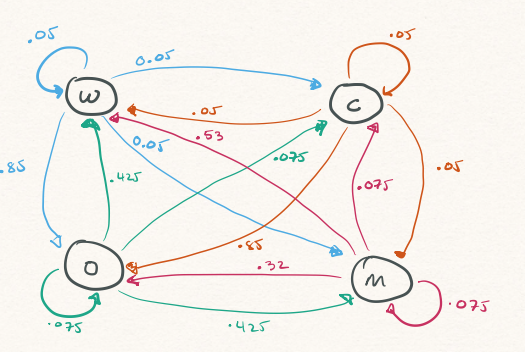
Imagine a bandwagon fan who randomly switches their support each day between four teams (W, O, M, and C) according to the transition probabilities in Figure 1. For instance, if they currently support W today, tomorrow they will support
- Team
Wwith probability 0.05 (i.e., they stay at vertexW) - Team
Mwith probability 0.05 (i.e., they move from vertexWto vertexM) - Team
Owith probability 0.85 (i.e., they move from vertexWto vertexO) - Team
Cwith probability 0.05 (i.e., they move from vertexWto vertexC)
Once the fan selects their new team to support, the process begins again: based on their current favorite team, they pick a new team based on the weights if the outgoing edges from the corresponding vertex in the graph.
The following code defines a function that simulates the Markov chain describing the fans behavior. The function takes three arguments: the starting state (i.e., the team the fan initially supports); the number of iterations to simulate; and the transition matrix \(\boldsymbol{\mathbf{P}}.\) It then returns the relative proportion of times that the chain spends in each state (i.e., how often the fan supports each team).
Now we define the matrix \(\boldsymbol{\mathbf{P}}\) correspond to the graph in Figure 1
teams <- c("W", "O", "C", "M")
P <- matrix(c(0.05, 0.85, 0.05, 0.05,
              0.425, 0.075, 0.075, 0.425,
              0.05, 0.85, 0.05, 0.05,
              0.53, 0.32, 0.075, 0.075),
            byrow = TRUE, nrow = 4, ncol = 4,
            dimnames = list(teams, teams))

set.seed(479)
round(fan_walk(init_state = "W", n_iter = 1e6, P = P), digits = 3)
states_visited
W O C M
0.307 0.416 0.066 0.211 round(fan_walk(init_state = "O", n_iter = 1e6, P = P), digits = 3)states_visited
W O C M
0.307 0.416 0.066 0.211 round(fan_walk(init_state = "C", n_iter = 1e6, P = P), digits = 3)states_visited
W O C M
0.307 0.416 0.066 0.211 round(fan_walk(init_state = "M", n_iter = 1e6, P = P), digits = 3)states_visited
W O C M
0.308 0.416 0.066 0.211 The long-run frequency that the chain spends in each state is remarkably stable: regardless of their initial preference, the fan spends about 30% of their time supporting W; 42% of the time supporting O; 7% of the time supporting C; and 21% of the time supporting M.
Limiting Distributions of Markov Chains
The stability in the long-run proportion of time spent in each state in the four-team example is not coincidental!
Distribution of \(X_{n}\)
Suppose that \(\{X_{t}\}\) is a Markov chain defined on the states \(\{1, 2, \ldots, S\}\) with transition matrix \(\boldsymbol{\mathbf{P}}.\) Let \(\boldsymbol{\pi}_{0} = (\pi_{0,1}, \ldots, \pi_{0,S})^{\top}\) be a vector of probabilities. Now suppose that we initialize the Markov chain randomly according to \(\boldsymbol{\pi}_{0}.\) That is, for each state \(s \in \{1, 2, \ldots, S\},\) \(\mathbb{P}(X_{0} = s) = \pi_{0,s}.\) If we initialize the Markov chain according to \(\boldsymbol{\pi}_{0}\) and then simulate the Markov chain for \(n\) steps, what is the probability that the chain is in state \(s\) after \(n\) steps?
Before jumping into the general case for the \(n\)-th visited step, we’ll start by carefully computing the distribution of the first visited state (i.e., \(X_{1}\)). To this end, observe that \[ \mathbb{P}(X_{1} = s') = \sum_{s}{\mathbb{P}(X_{1} = s' \textrm{ and } X_{0} = s)}, \] where the sum is taken over the entire state space \(\{1, 2, \ldots, S\}.\) We can further compute each summand in as the product of atransition probability and an initial probability: \[ \mathbb{P}(X_{1} = s' \textrm{ and } X_{0} = s) = \mathbb{P}(X_{1} = s' \vert X_{0} = s)\mathbb{P}(X_{0} = s). \] Since we know \(\mathbb{P}(X_{0} = s) \pi_{0,s}\) and \(\mathbb{P}(X_{1} = s' \vert X_{0} = s) = p_{s,s'},\) we conclude that \[ \mathbb{P}(X_{1} = s') = \sum_{s}{\pi_{0,s}p_{s,s'}} \] If we let if \(\boldsymbol{\pi}_{1} = (\pi_{1,1}, \ldots, \pi_{1,S})^{\top}\) where \(\pi_{1,s} = \mathbb{P}(X_{1} = s)\) be the probability distribution of \(X_{1},\) we can re-write the above equation in matrix form as \[ \boldsymbol{\pi}_{1}^{\top} = \boldsymbol{\pi}_{0}^{\top}\boldsymbol{\mathbf{P}} \] Using essentially the same calculation, we conclude that for each \(n\), \[ \boldsymbol{\pi}_{n}^{\top} = \boldsymbol{\pi}_{n-1}^{\top}\boldsymbol{\mathbf{P}}, \] where \(\boldsymbol{\pi}_{n} = (\pi_{n,1}, \ldots, \pi_{n,S})^{\top}\) and \(\pi_{n,s} = \mathbb{P}(X_{n} = s).\) Recalling the definition of the \(n\)-step transition probability matrix \(\boldsymbol{\mathbf{P}}^{(n)}\) from Lecture 14, we have \[ \boldsymbol{\pi}_{n}^{\top} = \boldsymbol{\pi}_{0}^{\top}\boldsymbol{\mathbf{P}}^{n}, \]
Invariant Distributions
Returning to the 4 team example from Figure 1, suppose that the bandwagon fan choose the initial team to support uniformly at random. The following code computes \(\boldsymbol{\pi}_{1}, \ldots, \boldsymbol{\pi}_{10}\)
pi0 <- rep(0.25, times = 4)
state_probs <- matrix(nrow = 10, ncol = 4, dimnames = list(c(), teams))
state_probs[1,] <- pi0
for(i in 2:10){
state_probs[i,] <- state_probs[i-1,] %*% P
}
round(state_probs, digits = 2)- 1
-
The \(i\)-th row of
state_probsholds the entries in the vector \(\boldsymbol{\pi}_{i-1}\) (i.e., the distribution of \(X_{i-1}\)).
         W    O    C    M
 [1,] 0.25 0.25 0.25 0.25
 [2,] 0.26 0.52 0.06 0.15
 [3,] 0.32 0.36 0.07 0.25
 [4,] 0.31 0.43 0.07 0.19
 [5,] 0.31 0.41 0.07 0.22
 [6,] 0.31 0.42 0.07 0.21
 [7,] 0.31 0.42 0.07 0.21
 [8,] 0.31 0.42 0.07 0.21
 [9,] 0.31 0.42 0.07 0.21
[10,] 0.31 0.42 0.07 0.21
We notice that after about four or five iterations, it appears that the vectors \(\boldsymbol{\pi}_{n-1}\) and \(\boldsymbol{\pi}_{n}\) are essentially identical. We observe the same phenomenon using a very different initial distribution
pi0 <- c(0.9, 0.05, 0.025, 0.025)
state_probs <- matrix(nrow = 10, ncol = 4, dimnames = list(c(), teams))
state_probs[1,] <- pi0
for(i in 2:10){
  state_probs[i,] <- state_probs[i-1,] %*% P
}
round(state_probs, digits = 2)
W O C M
[1,] 0.90 0.05 0.03 0.03
[2,] 0.08 0.80 0.05 0.07
[3,] 0.38 0.19 0.07 0.35
[4,] 0.29 0.51 0.06 0.13
[5,] 0.31 0.38 0.07 0.25
[6,] 0.31 0.42 0.07 0.20
[7,] 0.30 0.42 0.07 0.21
[8,] 0.31 0.41 0.07 0.21
[9,] 0.31 0.42 0.07 0.21
[10,] 0.31 0.42 0.07 0.21It would appear that if every \(\boldsymbol{\pi}_{n} \approx (0.31, 0.42, 0.07, 0.21)^{\top},\) then \(\boldsymbol{\pi}_{n+1} \approx \boldsymbol{\pi}_{n}.\) In other words, after a while, the uncertainty about what state the Markov chain is in appears to be invariant.
Definition: Invariant Distribution
Suppose \(\{X_{t}\}\) is a Markov chain over state space \(\{1, 2, \ldots, S\}\) with transition probability matrix \(\boldsymbol{\mathbf{P}}.\) The probability distribution \(\boldsymbol{\pi} = (\pi_{1}, \ldots, \pi_{S})^{\top}\) is invariant to \(\boldsymbol{\mathbf{P}}\) if \[ \boldsymbol{\pi}^{\top}\boldsymbol{\mathbf{P}} = \boldsymbol{\pi}. \] Notice that if \(\boldsymbol{\pi}\) is invariant, if the chain is initialized according to \(\boldsymbol{\pi}\) then \(\mathbb{P}(X_{t} = s) = \pi_{s}\) for all time steps \(t.\)
It turns out that for a broad class of Markov chains — specifically, those that are positive recurrent1, aperiodic2, and irreducible3 — then
- There is a unique invariant distribution \(\boldsymbol{\pi}\) satisfying \(\boldsymbol{\pi}^{\top}\boldsymbol{\mathbf{P}} = \boldsymbol{\pi}.\)
- As \(n \rightarrow \infty,\) $_{n} .
Computing Invariant Distributions
That is, under suitable conditions, the limiting distribution of the states visited by the Markov chain converges to the invariant distribution. This means that in order to determine the long-run frequency of the chain being in state \(s,\) we do not actualy have to simulate the Markov chain. Instead, we need find a probability vector \(\boldsymbol{\pi}\) such that \(\boldsymbol{\pi}^{\top}\boldsymbol{\mathbf{P}} = \boldsymbol{\pi}^{\top}.\) This relation implies that in fact, the invariant probability vector is a left eigenvector of the matrix \(\boldsymbol{\mathbf{P}}\) with eigenvalue 1. The following code defines a function that return the invariant distribution given a transition matrix \(\boldsymbol{\mathbf{P}}.\)
Function to compute leading left eigenvector of transition matrix
get_invariant <- function(P, tol = 1e-12){
states <- colnames(P)
if(!all( abs(rowSums(P) - 1) < tol) ){
stop("Rows sums of P are not all 1. P may not be a valid transition matrix") #<2
}
decomp <- eigen(t(P))
pi_raw <- decomp$vectors[,1]
if(!all(Re(pi_raw) < tol)){
stop("Leading eigenvalue of P appears to be complex and not real-valued")
}
pi <- Re(pi_raw)
pi <- pi/sum(pi)
names(pi) <- states
return(pi)
}- 1
-
When doing linear algebra in R, it’s helpful to work up to some degree of numerical precision. For most of our calculations, it’ll be enough to use
1e-12or1e-9 - 2
-
Transition matrices have row sums of 1. This checks that the row sums of the provided matrix
Pare sufficiently close to 1. If they are not, the function throws an error - 3
-
By default
eigen()returns right eigenvectors. The left eigenvectors of a matrix \(M\) are the right eigenvector of its transpose \(M^{\top}\) - 4
-
eigen()scales eigenvectors to have squared norm 1 and not a sum of 1. We need to re-scale this vector. - 5
-
Generally speaking, the eigenvalues and eigenvectors of a transition matrix are complex-valued and not real-valued. For a Markov chain with a limiting, invariant distribution the leading eigenvector should only have real values. This code checks that the imaginary parts are 0 (or at least smaller than than our small tolerance
tol)
As an illustration, in the code below we first compute the invariant distribution for our 4-team Markov chain. Then, we look at the different \(\boldsymbol{\pi}^{\top} - \boldsymbol{\pi}^{\top}\boldsymbol{\mathbf{P}}.\) We find that that differences are all of the other \(10^{-16},\) which for our purposes are small enough to be considered zero.
pi <- get_invariant(P)
cat("pi:", round(pi, digits = 6), "\n")
pi: 0.307308 0.415808 0.065675 0.211208 cat("pi %*% P:", round(pi %*% P, digits = 6), "\n")pi %*% P: 0.307308 0.415808 0.065675 0.211208 cat("Difference: ", pi - pi %*% P, "\n")Difference: -5.551115e-17 -2.220446e-16 1.387779e-17 2.220446e-16 If we interpret the bandwagon fans’ transitions from team \(s\) to \(s'\) to signify that team is \(s'\) is, in some sense, better than \(s,\) then we can rank teams by the amount of time the fan spends support thing. In our 4-team example, the bandwagon fan supports:
Wabout 30% of the timeOabout 42% of the timeCabout 7% of the timeMabout 21% of the time.
So, we would obtain the ranking O, W, M, and C based on this specific Markov chain.
Markov chain-based Rankings
We’re now in a position to apply this general procedure to our D1 hockey data. The main steps involve:
- Construct a Markov chain model describing how a bandwagon fan could randomly switch their support from team to team
- Compute the invariant distribution of the Markov chain
There are many ways to carry out the first step and there is no objective or normative best way to do so. By convention, we usually set up the Markov chain model so that \(p_{s,s'}\), the probability that the fan switches their support from \(s\) to \(s'\), quantifies how much better \(s'\) is than \(s.\) Most often, \(p_{s,s'}\) is selected to depend on the number of times \(s'\) beats \(s\) and/or the number of points \(s'\) scores against \(s.\)
Before proceeding, we will load in the data table constructed in Lecture 12 containing match-by-match results from the 2024-25 D1 Women’s Ice Hockey Season
load("wd1hockey_regseason_2024_2025.RData")
teams <- sort(unique(c(no_ties$Home, no_ties$Opponent)))
S <- length(teams)
results <-
no_ties |>
dplyr::rename(
home.team = Home, home.score = HomeScore,home.winner = Home_Winner,
away.team = Opponent, away.score = OppScore, away.winner = Opp_Winner) |>
dplyr::select(home.team, away.team, home.winner, away.winner, home.score, away.score)- 1
- Vector containing the list of all teams
- 2
- Number of teams
- 3
- Rename columns in original table and extract home and away team identities, scores, and indicators for winning
Damping
Suppose that our bandwagon fan currently supports team \(s\) and must now (randomly) select another team \(s'\) to support. Since we’d like for our fan to more often move to “better” teams, it makes sense to send the fan from \(s\) to \(s'\) than to another team \(t\) if more frequently if \(s'\) has beaten \(s\) more often than \(t\) has beaten \(s.\) To formalize this intuition, we begin by creating a matrix \(\boldsymbol{\mathbf{V}}\) whose \((s,s')\) element \(v_{s,s'}\) counts the number of times \(s'\) beats \(s.\)
V <- matrix(0, nrow = S, ncol = S, dimnames = list(teams, teams))
for(i in 1:nrow(results)){
home <- results$home.team[i]
away <- results$away.team[i]
if(results$home.winner[i] == 1){
V[away,home] <- V[away,home] + 1
} else if(results$away.winner[i] == 1){
V[home,away] <- V[home,away] + 1
} else{
cat("Problem with game", i, ": neither team won")
}
}- 1
- Initialize \(\boldsymbol{\mathbf{V}}\) to have all zero entries
- 2
-
The
V[away,home]counts how many timeshomebeataway. So, every time the home team wins a game, we must incrementV[away,home]. - 3
-
The
V[home,away]counts how many timesawaybeathome. So, every time the away team wins a game, we must incrementV[home,away]. - 4
- This condition should never be reached, since we removed ties from the data back in Lecture 12
Each row of a transition probability matrices must sum to 14. In its present form, \(\boldsymbol{\mathbf{V}}\) does not satisfy this property: in fact, the row and columns sums of \(\boldsymbol{\mathbf{V}}\) respectively count the number of losses and wins for each team. To turn \(\boldsymbol{\mathbf{V}}\) into a valid transition probability matrix, we need to normalize the rows.
Mathematically, let \(\mathbf{\boldsymbol{A}}\) be the \(S \times S\) diagonal matrix whose \((s,s')\) entry is zero for all \(s \neq s\) and whose \((s,s)\) entry, \(a_{s,s}\), is sum of the elements along the \(s\)-th row of \(\boldsymbol{\mathbf{V}}\): \[a_{s,s} = \sum_{s'}{v_{s,s'}}\] Then, the matrix \(\boldsymbol{\mathbf{W}} = \boldsymbol{\mathbf{A}}^{-1}\boldsymbol{\mathbf{V}}\) is the row-normalized version of \(\boldsymbol{\mathbf{V}}.\)
r <- rowSums(V)
if(any(r == 0)) r[r==0] <- 1
A <- diag(x = r)
W <- solve(A) %*% V
dimnames(W) <- dimnames(V)- 1
-
If any rows of
Vhave a sum of zero (e.g., for an undefeated team), we will set the corresponding element ofAto be 1 so that the corresponding row ofWcontains only zeros. - 2
-
diag()creates a diagonal matrix with diagonal entries given by - 3
-
solve()returns the inverse of a matrix.
Since the rows of \(\boldsymbol{\mathbf{W}}\) sum to one, it is tempting to use it as the transition matrix for our Markov chain. There are a few issues with that, however. To illustrate them, we first look at the rows and columns of \(\boldsymbol{\mathbf{W}}\) corresponding to the teams who qualified for the 2024-25 Frozen 4
W[c("Wisconsin", "Ohio State", "Cornell", "Minnesota"), c("Wisconsin", "Ohio State", "Cornell", "Minnesota")] Wisconsin Ohio State Cornell Minnesota
Wisconsin 0.0000000 1.00 0 0.00
Ohio State 0.2500000 0.00 0 0.25
Cornell 0.0000000 0.20 0 0.00
Minnesota 0.4166667 0.25 0 0.00If we simulated a Markov chain using transitions in \(\boldsymbol{\mathbf{W}},\) then the chain would always move from Wisconsin to Ohio State (since Ohio State was the only team to beat Wisconsin last season). While this is subjectively bad, the more serious issue is that it turns out the Markov chain so defined is not necessarily aperiodic, positive recurrent, and irreducible. So, it may not always have A somewhat less abstract issue is that all diagonal elements of \(\boldsymbol{\mathbf{W}}\) are zero. This means that the bandwagon fan who switches their support sequentially according to \(\boldsybmol{\mathbf{W}}\) never has the option to stick with the same team across multiple rounds.
To overcome this issue, it is common to introduce a damping factor as follows. First, one fixes a number \(0 < \beta < 1\) (e.g., \(\beta = 0.5\) or \(\beta = 0.85\)) and then creates a transition matrix \[ \boldsymbol{\mathbf{P}} = \beta \times \boldsymbol{\mathbf{W}} + \frac{(1 - \beta)}{S} \times \mathbf{\boldsymbol{1}}_{S}^{\top}\mathbf{\boldsymbol{1}}_{S} \] by
- Scaling all the elements of \(\boldsymbol{\mathbf{W}}\) by \(\beta\)
- Adding \((1-\beta)/S\) to every element of the re-scaled matrix (both off-diagonal and diagonal elements)
Doing so ensures that the matrix is irreducible, aperiodic, and positive recurrent, which means that \(\boldsymbol{\mathbf{P}}\) has a unique limiting, invariant distribution. So, if we simulate a bandwagon fan switching their support between teams according to \(\boldsymbol{\mathbf{P}},\) we can derive a rank ordering of teams from the long-run proportion of time they spend supporting each team.
In the following code, we define a function that takes a matrix \(\boldsymbol{\mathbf{V}}\) and damping factor \(\beta\) and outputs the resulting transition matrix \(\boldsymbol{\mathbf{P}}.\)
get_dampened_transition <- function(V, beta){
  states <- rownames(V)
  n_states <- nrow(V)

  r <- rowSums(V)
  if(any(r == 0)) r[r==0] <- 1
  A <- diag(r)
  W <- solve(A) %*% V
  P <- beta * W + (1-beta)/n_states
  dimnames(P) <- dimnames(V)
  return(P)
}
Simulating the random walk behavior of our bandwagon fan beginning at Wisconsin, we find that the fan spends about 11% of the time supporting Ohio State, 8% of the time supporting Wisconsin, and 6% of the time supporting Minnesota.
P <- get_dampened_transition(V, beta = 0.85)
sim1 <- fan_walk(init_state = "Wisconsin", n_iter = 1e6, P = P)
round(sort(sim1, decreasing = TRUE), digits = 3)[1:10]
states_visited
Ohio State Wisconsin Minnesota Minnesota Duluth
0.114 0.080 0.059 0.046
Cornell Colgate Northeastern St. Cloud State
0.040 0.039 0.032 0.031
St. Lawrence Penn State
0.028 0.026 Reassuringly, these long-run frequency estimates are very close to the invariant distribution of \(\boldsymbol{\mathbf{P}}\)
pi <- get_invariant(P)
round(sort(pi, decreasing = TRUE), digits = 3)[1:10]
Ohio State Wisconsin Minnesota Minnesota Duluth
0.115 0.080 0.059 0.046
Cornell Colgate Northeastern St. Cloud State
0.040 0.039 0.032 0.032
St. Lawrence Connecticut
0.028 0.026 Score-based Markov Chain Rankings
Based on the particular model of bandwagon fan behavior from the previous section, we obtain a power ranking in which Ohio State is first and Wisconsin is second. This is despite the fact that (i) Wisconsin beat most of its opponents in the 2024-25 regular season and (ii) Wisconsin won more games than Ohio State. Remember, we constructed the Markov chain so that the fan would move from team \(s\) to team \(s'\) more often the more times \(s'\) beat \(s.\) Since Wisconsin only lost to Ohio State and to nobody else, our Markov chain model specifies a rather large transition probability from Wisconsin to Ohio State.
Another, somewhat less subjective objection to the model, lies in the fact that transitions only depend on match results and not on the scoring margin or the number of goals scored. As a refinement, let’s try to build a different \(\boldsymbol{\mathbf{V}}\) that takes scoring into account. Specifically, we will set \(v_{s,s'}\) equal to the total number of points scored by \(s'\) when it plays \(s.\) In our hockey context, the row and column sums of this new \(\boldsymbol{\mathbf{V}}\) are, respectively, the number of goals conceded and number of goals scored by each team.
V_score <- matrix(0, nrow = S, ncol = S, dimnames = list(teams, teams))
for(i in 1:nrow(results)){
home <- results$home.team[i]
away <- results$away.team[i]
V_score[away, home] <- V_score[away,home] + results$home.score[i]
V_score[home,away] <- V_score[home,away] + results$away.score[i]
}- 1
-
Re-initialize
Vto have all entries equal to 0 - 2
-
Add the number of goals scored by the home team when playing the away team to
V[away,home] - 3
-
Add the number of goals scored by the away team when playing the home team to
V[home,away].
We now convert our score-based \(\boldsymbol{\mathbf{V}}\) into a dampened transition matrix with \(\beta = 0.8\) and then compute the resulting invariant distribution. Now, it appears that Wisconsin is at the top of the power rankings, closely followed by Minnesota and Ohio State.
P_score <- get_dampened_transition(V_score, beta = 0.8)
pi_score <- get_invariant(P_score)
round(sort(pi_score, decreasing = TRUE), digits = 3)[1:10]
Wisconsin Minnesota Ohio State Colgate
0.053 0.048 0.045 0.039
Cornell Minnesota Duluth Minnesota State Clarkson
0.034 0.033 0.030 0.029
St. Lawrence Princeton
0.029 0.028 Guest Speaker
- Thursday October 30: David Radke (Chicago Blackhawks)
- 2:30pm - 3:30pm: Research Talk
- “Multiagent Challenges in Team Sports Analytics”
- Aimed at graduate students & faculty but all welcome!
- 3:30pm - 4:30pm: Career Talk
- “Professional Hockey Analytics at the Chicago Blackhawks”
- How does Hockey Strateegy & Analytics groups operate?
- Both talks in Morgridge Hall 7560
Footnotes
A chain is said to be positive recurrent if for all states \(s,\) a chain begun in \(s\) is guaranteed to return to \(s\) in a finite number of steps with probability 1. A sufficient (but not necessary) condition is for \(p_{s,s} > 0\) for all states \(s.\)↩︎
The period of state \(s\) is the greatest common divisor of all \(n\) such that \((\boldsymbol{P}^{n})_{s,s} > 0.\) If state \(s\) has period \(d,\) this means that the chain has non-zero probability of returning to \(s\) every \(d\) steps. An aperiodic chain is one in which the period of every state is 1. That is, in an aperiodic chain, there is always a chance of returning to the same state in one step.↩︎
Informally, irreducible Markov chains are those in which there is a any state \(s'\) can be reached from any other state in a finite number of steps. A sufficient (but not necessary) condition is that \(p_{s,s'} > 0\) for all pairs of state \(s\) and \(s'\)↩︎
Remember, the \(s\)-th row of \(\boldsymbol{\mathbf{P}}\) specifies a distribution of the state the Markov chain visits immediately being in state \(s.\) Since the chain must move (or remain in \(S\)), the sum of the probabilities along the rows has to be 1.↩︎