install.packages("hoopR")Lecture 4: Adjusted Plus/Minus
Overview
Which NBA players do the most to help their teams win? And how might we quantify that contribution? One option is to rely on box score statistics like points, rebounds, assists, steals, blocks, and turnovers. Underlying this approach is the assumption that the “best” or players with the most impact are the ones that record extreme values of these statistics. That is, they are the ones who score the most points, grab the most rebounds, commit the fewest turnovers, etc?
While this approach seems natural, it quickly runs into problems. As Ilardi 2007 notes, it is not obvious whether all of these statistics should count the same or whether some should be weighted more heavily than others. It is also difficult to compare players who play different roles: is a guard who records 10 assists per game more valuable than a center who grabs 10 rebounds per game? More subtley, players do many things during the course of a game (e.g., setting screens, rotating on defense, dive for loose balls, etc.) that impact the outcome of a play or the game but do not appear in the box score. How should those contributions be valued?
In today’s lecture, we introduce two now-classical approaches to player evaluation: plus/minus (Section 3) and adjusted plus/minus (Section 4). At a high-level, plus/minus is simply the total point differential that a player’s team accrues when he is on the court. Adjusted plus/minus measures how much more a player contributes to his team’s point differential per 100 after accounting than a baseline-level player, after accounting for the relative contributions of his teammates and opponents.
Stint-Level NBA Data
To compute plus/minus and adjusted plus/minus, we need to build a data table in which rows correspond to stints within individual games. In addition to recording the identities of the home and away team players on the court during each stint, the data table needs to include game-state information about each stint including both teams’ scores and the amount of time left at the start and end of each stint and the number of possessions in each stint. Such a table can be built using play-by-play data.
The NBA posts a play-by-play for every game containing the time-stamp and a short description of important events during a game. Basically, whenever a player does something tracked by the scorekeepers or reported in the box-score (e.g., attempt a shot, steal the ball, commit a foul, etc.), an entry is added to the play-by-play log. Here is an example from a game from a few years ago between the Dallas Mavericks and Minnesota Timberwolves1.
We can scrap play-by-play data into R using the [hoopR] package, which can be installed using the code:
The following function, which is based on a script written by Ron Yurko, extracts stint information from a single game’s play-by-play.
Warning
It takes about 30 minutes to download all single season’s worth of play-by-play data.
Show code to get stint data
get_game_stint_data <- function(game_i) {
game_data <- hoopR::nba_pbp(game_id = game_i)
game_data$home_score[1] <- 0
game_data$away_score[1] <- 0
game_data$score_margin[1] <- 0
game_data <-
game_data |>
tidyr::fill(home_score, away_score, score_margin)
home_lineups <-
game_data |>
dplyr::select(home_player1, home_player2, home_player3, home_player4, home_player5) |>
apply(MARGIN = 1, FUN = function(x){paste(sort(x), collapse = "_")})
away_lineups <-
game_data |>
dplyr::select(away_player1, away_player2,away_player3, away_player4, away_player5) |>
apply(MARGIN = 1, FUN = function(x){paste(sort(x), collapse = "_")})
game_data$home_lineup <- home_lineups
game_data$away_lineup <- away_lineups
# Now there are a couple of ways to figure out the stints, but I think the
# best way is to use the substitution events - where a stint changes once
# a substitution takes places (but only if the previous event was NOT a substitution)
# Start by making an indicator for the stint change:
game_data <-
game_data |>
dplyr::mutate(is_sub = ifelse(event_type == 8, 1, 0),
new_stint_start = ifelse((is_sub == 1) & (dplyr::lead(is_sub) != 1),1, 0))
# For substitutions that take place
# during a free throw window, then the new stint should start after the free throw
# Easiest way to track if substitution takes places before final free throw:
game_data <-
game_data |>
dplyr::mutate(sub_during_free_throw = dplyr::case_when(
(stringr::str_detect(visitor_description, "Free Throw 1 of 1") |
stringr::str_detect(visitor_description, "Free Throw 2 of 2") |
stringr::str_detect(visitor_description, "Free Throw 3 of 3")) &
(dplyr::lag(is_sub) == 1) ~ 1,
(stringr::str_detect(home_description, "Free Throw 1 of 1") |
stringr::str_detect(home_description, "Free Throw 2 of 2") |
stringr::str_detect(home_description, "Free Throw 3 of 3")) &
(dplyr::lag(is_sub) == 1) ~ 1,
.default = 0),
# Now if the sub is followed by this, then set new_stint_start to 0, but
# if this set a new stint to start post the final free throw:
new_stint_start = ifelse(is_sub == 1 & dplyr::lead(sub_during_free_throw) == 1, 0, new_stint_start),
new_stint_start = ifelse(lag(sub_during_free_throw) == 1,1, new_stint_start),
new_stint_start = ifelse(is.na(new_stint_start), 0, new_stint_start)
)
# Filter out subs that are not new stints, and then just use
# the cumulative sum of the new stint start to effectively create a stint ID:
game_data <- game_data |>
dplyr::filter(!(is_sub == 1 & new_stint_start == 0)) |>
dplyr::mutate(stint_id = cumsum(new_stint_start) + 1)
# Toughest part - need to count the number of possessions for each team during
# the stint... will rely on this for counting when a possession ends:
# https://squared2020.com/2017/09/18/deep-dive-on-regularized-adjusted-plus-minus-ii-basic-application-to-2017-nba-data-with-r/
# "Recall that a possession is ended by a converted last free throw, made field goal, defensive rebound, turnover, or end of period"
game_data <- game_data |>
dplyr::mutate(pos_ends = dplyr::case_when(
stringr::str_detect(home_description, " PTS") &
stringr::str_detect(home_description, "Free Throw 1 of 2", negate = TRUE) &
stringr::str_detect(home_description, "Free Throw 2 of 3",negate = TRUE) ~ 1, # made field goals or free throws
stringr::str_detect(visitor_description, " PTS") &
stringr::str_detect(visitor_description, "Free Throw 1 of 2",negate = TRUE) &
stringr::str_detect(visitor_description, "Free Throw 2 of 3",negate = TRUE) ~ 1,
stringr::str_detect(tolower(visitor_description), "rebound") &
stringr::str_detect(tolower(lag(home_description)), "miss ") ~ 1,
stringr::str_detect(tolower(home_description), "rebound") &
stringr::str_detect(tolower(lag(visitor_description)), "miss ") ~ 1,
stringr::str_detect(tolower(home_description), " turnover") ~ 1,
stringr::str_detect(tolower(visitor_description), " turnover") ~ 1,
stringr::str_detect(neutral_description, "End") ~ 1,.default = 0))
# Now the final part - compute the stint level summaries:
game_data |>
dplyr::group_by(stint_id) |>
dplyr::summarize(
home_lineup = dplyr::first(home_lineup),
away_lineup = dplyr::first(away_lineup),
n_home_lineups = length(unique(home_lineup)),
n_away_lineups = length(unique(away_lineup)),
start_home_score = dplyr::first(home_score),
end_home_score = dplyr::last(home_score),
start_away_score = dplyr::first(away_score),
end_away_score = dplyr::last(away_score),
start_minutes = dplyr::first(minute_game),
end_minutes = dplyr::last(minute_game),
n_pos = sum(pos_ends),
.groups = "drop") |>
dplyr::mutate(
home_points = end_home_score - start_home_score,
away_points = end_away_score - start_away_score,
minutes = end_minutes - start_minutes,
pts_diff = home_points - away_points,
margin = 100 * (pts_diff) / n_pos,
game_id = game_i) |>
dplyr::select(game_id, stint_id,
start_home_score, start_away_score,
start_minutes,
end_home_score, end_away_score, end_minutes,
home_lineup, away_lineup, n_pos,
home_points, away_points, minutes, pts_diff, margin) |>
dplyr::filter(n_pos != 0)
}
poss_get_game_stints <-
purrr::possibly(.f = get_game_stint_data, otherwise = NULL)- 1
- Function to extract the stints from a single game’s play-by-play
- 2
- Initialize the starting score and margin (i.e., point differential per 100 possessions) at 0
- 3
-
tidyr::fill()fills in missing values with the previous entry. - 4
- Get the 5 home team players and a create a string of the numeric IDs separated by underscores (“_“)
- 5
- Get the 5 away team players and a create a string of the numeric IDs separated by underscores (“_“)
- 6
-
Add the strings recording who is on the court to
game_data - 7
- Compute number of points scored by each team and other game-state information
- 8
- Remove stints with 0 possessions.
- 9
-
We will loop over many games. To prevent an error from prematurely terminating the loop (e.g., from a game with missing or corrupted play-by-play), we create a version that returns
NULLwhen it hits an error.
The following code downloads play-by-play logs for every game in the 2024-25 season and applies the function defined above to create our stint-level data table.
raw_game_log <- hoopR::nba_leaguegamelog(season = 2024)
nba_game_log <- raw_game_log$LeagueGameLog
nba_season_games <-
nba_game_log |>
dplyr::pull(GAME_ID) |>
unique()
season_stint_data <-
purrr::map(nba_season_games, ~poss_get_game_stints(.x)) |>
dplyr::bind_rows()
game_stint_context <-
season_stint_data |>
dplyr::select(
game_id, stint_id, n_pos,
start_home_score, start_away_score,start_minutes,
end_home_score, end_away_score, end_minutes,
home_points, away_points, minutes,
pts_diff, margin)
home_players_data <-
season_stint_data |>
dplyr::select(game_id, stint_id, home_lineup)|>
tidyr::separate_rows(home_lineup, sep = "_") |>
dplyr::mutate(on_court = 1) |>
tidyr::pivot_wider(
id_cols = c("game_id", "stint_id"),
names_from = home_lineup,
values_from = on_court,
values_fill = 0)
home_players_cols <- colnames(home_players_data)[3:ncol(home_players_data)]
away_players_data <-
season_stint_data |>
dplyr::select(game_id, stint_id, away_lineup) |>
tidyr::separate_rows(away_lineup, sep = "_") |>
dplyr::mutate(on_court = -1) |>
tidyr::pivot_wider(
id_cols = c("game_id", "stint_id"),
names_from = away_lineup,
values_from = on_court,
values_fill = 0)
away_players_cols <- colnames(away_players_data)[3:ncol(away_players_data)]
game_stint_players_data <-
home_players_data |>
dplyr::bind_rows(away_players_data) |>
dplyr::group_by(game_id, stint_id) |>
dplyr::summarize(
dplyr::across(dplyr::everything(), ~ sum(.x, na.rm = TRUE)),
.groups = "drop")
rapm_data <-
game_stint_context |>
dplyr::left_join(game_stint_players_data,by = c("game_id", "stint_id"))- 1
- Get the ID number for every game
- 2
- Loop over all game IDs and extract stint information
- 3
-
purrr::map()stores the stint data table for each game as a separate element of a list. Here we concatenate each of these tables into a single table. - 4
- Pulls out the game-state/contextual information about each stint
- 5
- Creates a column for every home team player’s on-court indicator
- 6
- Creates a column for every away team player’s on-court indicator
- 7
- Concatenates the home team indicators and away team indicators
- 8
- Joins the player on-court indicators with the contextual information about the stint
The first 14 columns of rapm_data record:
- Numeric identifiers for the game (
game_id) and stint (stint_id). - Both teams’ scores and the amount of time remaining at the start of a stint:
start_home_score,start_away_score, andstart_minutes. - Both teams’ scores and the amount of time remaining at the end of each stint:
end_home_score,end_away_score, andend_minutes. - The length of a stint (
minutes), the number of points scored by the home (home_points) and away team (away_points), and the number of possessions (n_pos). - The score differential
pts_diff = home_points - away_points. - The score differential per 100 possessions,
margin = pts_diff/n_pos * 100.
The remaining columns record whether individual players are not on the court (0), on the court and playing at home (+1), or on the court and playing on the road (-1) in each stint. The names of these columns are just identifiers assigned by hoopR. The function hoopR::nba_commonallplayers() returns a table with all players identifiers and names. The code below uses the function hoopR::nba_commonallplayers() to make a look-up table containing player names and identifiers. It also creates a column where all accents and special characters have been removed, which makes it easier to look up player ids by name (i.e., we can type “Luka Doncic” instead of “Luka Dončić”).
player_table <-
hoopR::nba_commonallplayers()[["CommonAllPlayers"]] |>
dplyr::select(PERSON_ID, DISPLAY_FIRST_LAST) |>
dplyr::rename(id = PERSON_ID, FullName = DISPLAY_FIRST_LAST) |>
dplyr::mutate(
Name = stringi::stri_trans_general(FullName, "Latin-ASCII"))- 1
-
The function returns a list with a single element named “CommonAllPlayers”. The
[[ ]]bit pulls out the table. - 2
- Transliterate player names to ASCII. Effectively this strips out the accents
Plus/Minus
Intuitively, we expect a team to perform better when a “good” player is on the court than when he is not on the court. Similarly, we expect a team to perform worse when a “bad” player is on the court than when he is not on the court. Plus/Minus (hereafter +/-) attempts to quantify this intuition by computing the total number of points by which a player’s team outscores their opponents when that player is on the floor. If a player has a large, positive +/- value, that means that the player’s team outscored its opponents by a large margin Similarly, a large, negative +/- value indicates that a player’s team was outscored by a wide margin when the player was on the court.
Computing Individual +/-’s
As an example, let’s compute the plus/minus values for Shai Gilgeous-Alexander (SGA), who was recognized as the league’s Most Valuable Player (MVP) in the 2024-25 regular season. To compute SGA’s +/-, we need to
- Sum the home team point differentials (i.e., the values in the column
pts_diff) for all stints where SGA was on the court and playing at home. - Sum the negative of the home team point differentials for all stints where SGA was on the court and playing on the road.
- Add the two totals from Steps 1 and 2.
Mathematically, for every stint \(i\) in our data table, let \(\Delta_{i}\) be the home team’s point differential during that stint. Additionally, let \(x_{i, \textrm{SGA}}\) be the signed on-court indicator that is equal to 1 if SGA is on the court and playing at home during stint \(i\); -1 if Shai is on the court and playing on the road during stint \(i\); and 0 if SGA is not on the court during stint \(i.\) Then, SGA’s +/- is equal to \[
\sum_{i = 1}^{n}{x_{i,\textrm{SGA}} \times \Delta_{i}}.
\] The data table rapm_data contains a column with the signed on-court indicators for every player. The names of these columns are just the hoopR identifiers, which were recorded in the id column of our look-up table player_table. The following code computes Shai’s +/- and uses the function [dplyr::pull()](https://dplyr.tidyverse.org/reference/pull.html) to extract values from specific columns of rapm_data.
shai_id <-
player_table |>
dplyr::filter(Name == "Shai Gilgeous-Alexander") |>
dplyr::pull(id)
shai_x <- rapm_data |> dplyr::pull(shai_id)
delta <- rapm_data |> dplyr::pull(pts_diff)
sum(shai_x * delta)- 1
- Find the row in our look-up table corresponding to SGA
- 2
-
Since there is only one row corresponding to SGA, this saves SGA’s identifier as
shai_id - 3
-
Extracts the vector of SGA’s signed on-court indicators from the corresponding column of
rapm_data - 4
-
Extracts the vector of home team point differentials across all stints from
rapm_data - 5
- Computes SGA’s +/-
[1] 888We now repeat this calculation for Nikola Jokic, who finished second in the MVP voting in the 2024-25 regular season. His overall +/- is substantially smaller than SGA’s.
jokic_id <-
  player_table |>
  dplyr::filter(Name == "Nikola Jokic") |>
  dplyr::pull(id)

jokic_x <- rapm_data |> dplyr::pull(jokic_id)
sum(jokic_x * delta)
[1] 452Matrix-Based Computation
Repeating this calculation for all players one at a time is exceptionally tedious. Luckily, with a bit of matrix algebra, we can compute the +/- for all players in one shot.
To this end, let \(n\) be the total number of stints in our data table and let \(p\) be the total number of players. Just like we did for SGA and Jokic in Section 3.1, for each stint \(i = 1, \ldots, n\) and for each player \(j = 1, \ldots, p,\) let \(x_{ij}\) be the signed on-court indicator for player \(j\) during stint \(i.\) So, \(x_{ij}\) is equal to 0 if player \(j\) is not on the court during stint \(i\) and is equal to 1 (resp. -1) if player \(j\) is on the court and playing at home (resp. on the road) during stint \(i.\) Player \(j\)’s overall +/- is given by \[ \sum_{i = 1}^{n}{x_{ij}\Delta_{i}}. \] We can arrange the \(x_{ij}\) values into an \(n \times p\) matrix \(\boldsymbol{\mathbf{X}}\) so that \(x_{ij}\) appears in in the \(j-th\) column of the \(i\)-th row (i.e., \(x_{ij}\) is the \((i,j)\) entry of \(\boldsymbol{\mathbf{X}}\)2). This way, the rows (resp. columns) of \(\boldsymbol{\mathbf{X}}\) correspond to stints (resp. players). Let \(\boldsymbol{\Delta}\) be the vector of length \(n\) whose \(i\)-th entry is \(\Delta_{i},\) the home-team point differential in stint \(i.\)
It turns out3 that player \(j\)’s +/- is the \(j\)-th entry of the vector obtained when we multiply the transpose[^transpose] of \(\boldsymbol{\mathbf{X}}\) by the vector \(\boldsymbol{\Delta}.\) That is, if \[ \boldsymbol{\mathbf{pm}} = \boldsymbol{\mathbf{X}}^{\top}\boldsymbol{\Delta}, \] then the vector \(\boldsymbol{\mathbf{pm}}\) contains \(p\) entries and its \(j\)-th entry is given by \[ \textrm{pm}_{j} = \sum_{i = 1}^{n}{x_{ij}\Delta_{i}}. \] [^transpose]: The transpose of a matrix \(\boldsymbol{A}\), which is denoted as \(\boldsymbol{A}^{\top}\), is obtained by switching the rows and columns indices. For instance, \(\begin{pmatrix} 1 & 2 & 3 \\ 4 & 5 & 6 \end{pmatrix}^{\top} = \begin{pmatrix} 1 & 4 \\ 2 & 5 \\ 3 & 6 \end{pmatrix}.\) See this Wikipedia article for more information.
The first 14 columns of the data table rapm_data contain contextual information about the stint. The remaining columns contain the values of each player’s signed on-court indicators. So, to form the matrix \(\boldsymbol{\mathbf{X}},\) we just need to drop the contextual columns.
context_vars <-
c("game_id", "stint_id", "n_pos",
"start_home_score", "start_away_score", "start_minutes",
"end_home_score", "end_away_score", "end_minutes",
"home_points", "away_points", "minutes",
"pts_diff", "margin")
X_full <-
as.matrix(
rapm_data |>
dplyr::select(- tidyr::all_of(context_vars)))- 1
-
Vector of contextual variables contained in
rapm_data - 2
-
Converts from a
tibbleto amatrix - 3
- Drops the contextual variables
In R, we can compute the transpose of a matrix using the function t(). But, it turns out that when we want to compute a product like \(\boldsymbol{\mathbf{X}}^{\top}\boldsymbol{\Delta},\) it is much more efficient to use the function crossprod().
The following code creates a data table pm with one column containing player id’s another column containing plus/minus values. It then uses an inner_join to append player names. The code also computes the number of possessions played by each player. To this end, let \(\textrm{pos}_{i}\) be the number of possessions played during stint \(i\). Notice that \(\lvert x_{ij} \rvert\) is equal to 1 whenever player \(j\) is on the court and is equal to 0 otherwise. So, the number of possessions played by player \(j\) is simply \(\sum_{i = 1}^{n}{\lvert x_{ij} \rvert \textrm{pos}_{i}}.\)
pm <-
data.frame(
id = colnames(X_full),
pm = crossprod(x = X_full, y = delta),
n_pos = crossprod(abs(X_full), y = rapm_data |> dplyr::pull(n_pos)),
minutes = crossprod(abs(X_full), y = rapm_data |> dplyr::pull(minutes))) |>
dplyr::inner_join(y = player_table |> dplyr::select(id, Name), by = "id") |>
dplyr::select(id, Name, pm, n_pos, minutes) |>
dplyr::arrange(dplyr::desc(pm))- 1
- Creates a column containing player ID’s
- 2
- Computes each player’s +/-.
- 3
-
Computes the number of possessions played by each player. The function
abs()computes absolute value. We useddplyr::pullto extract the number of possessions in each stint. - 4
- Compute the number of minutes played by each player.
- 5
-
Append only the names of players from
player_tablewhose ID appears as a column name ofX_full - 6
- Re-arrange the columns
Looking at the +/- values for a handful of selected players, we notice that SGA had a much higher +/- than many other prominent players in the league.
selected_players <-
  c("Shai Gilgeous-Alexander",
    "Jayson Tatum",
    "Nikola Jokic",
    "Giannis Antetokounmpo",
    "Luka Doncic",
    "Anthony Davis",
    "LeBron James")
pm |> dplyr::filter(Name %in% selected_players) |> dplyr::select(Name, pm)
Name pm
1 Shai Gilgeous-Alexander 888
2 Jayson Tatum 474
3 Nikola Jokic 452
4 Giannis Antetokounmpo 331
5 Luka Doncic 276
6 Anthony Davis -78
7 LeBron James -88The following code helps visualize just how much larger SGA’s +/- was compared to the rest of these selected players and the rest of the league.
oi_colors <- palette.colors(palette = "Okabe-Ito")
n <- nrow(X_full)
p <- ncol(X_full)
y_lim <- max(abs(pm$pm)) * c(-1.01, 1.01)
par(mar = c(3,3,2,1), mgp = c(1.8, 0.5, 0))
plot(1, type = "n",
xlim = c(0, p+1), ylim = y_lim,
xlab = "", xaxt = "n",
ylab = "+/-", main = "Plus-Minus")
for(i in 1:p){
lines(x = c(p+1-i,p+1-i), y = c(0, pm$pm[i]),
col = oi_colors[9], lwd = 0.25)
if(pm$Name[i] %in% selected_players){
points(x = p+1-i, y = pm$pm[i], pch = 16, cex = 0.7, col = oi_colors[3])
} else{
points(x = p+1-i, y = pm$pm[i], pch = 16, cex = 0.25, col = oi_colors[9])
}
}
abline(h = 0, col = oi_colors[8])- 1
- Load a color-blind friendly palette
- 2
- Handy to keep the number of stints and players in our environment
- 3
- To set symmetric vertical limits in our plot, we adjust the largest absolute +/- value by 1% in each direction.
- 4
- Tells R to set up the plot area but not to plot anything in it
- 5
- Set the horizontal and vertical limits of the plot.
- 6
- Suppresses the horizontal axis and its labels
- 7
- Label the vertical axis and add a title to the plot
- 8
-
The data table
pmis sorted with +/- in decreasing order. To visualize these values in increasing order, we plot the \(i\)-th largest +/- value at the horizontal coordinate \(p+1-i\). - 9
-
The argument
lwdcontrols the thickness of the lines. Setting it to 0.25 prevents over-plotting in this case
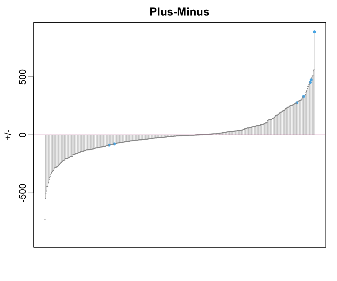
Issues with +/-
The gap SGA’s +/- and the +/- values for the rest of the league is striking. Is this gap really attributable to difference in skill alone? Or is the gap an artifact of some systematic factors? When we plot each player’s +/- against the number of possessions played, we find much more variation in the +/- values of players who played more possessions than those who played less.
par(mar = c(3,3,2,1), mgp = c(1.8, 0.5, 0))
plot(pm$n_pos, pm$pm,
     pch = 16, cex = 0.5, col = oi_colors[9],
     xlab = "Possessions played", ylab = "+/-",
     main = "Plus-Minus vs Possessions")
abline(h = 0, col = oi_colors[8])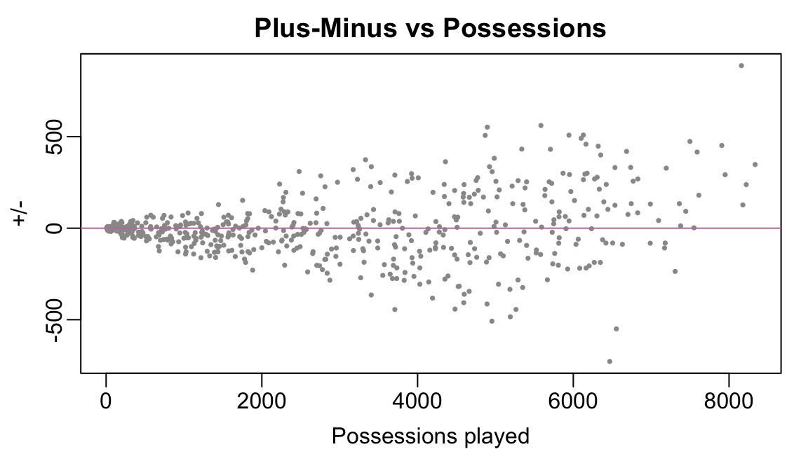
Because +/- is an aggregated statistic — that is, it is formed by adding up contributions over the course of a season — this is not wholly surprising. We see that SGA, in particular, played many more possessions than the other players with the ten highest +/- values. Consequently, if player A has a higher +/- than player B, we cannot immediately conclude that A is better or more valuable than B due to potential disparities in opportunities.
pm |> dplyr::slice_head(n=10) id Name pm n_pos minutes
1 1628983 Shai Gilgeous-Alexander 888 8159 2837.31
2 1629652 Luguentz Dort 561 5584 1955.17
3 1630198 Isaiah Joe 552 4896 1715.11
4 1628401 Derrick White 509 6129 2327.72
5 1630596 Evan Mobley 508 5944 2049.43
6 1630598 Aaron Wiggins 507 4868 1683.08
7 1628378 Donovan Mitchell 491 6101 2106.53
8 1628369 Jayson Tatum 474 7498 2840.95
9 1628386 Jarrett Allen 459 6163 2142.82
10 203999 Nikola Jokic 452 7907 2707.97Looking at the top-10 plus/minus values reveals another potential issue: three of SGA’s teammates (Dort, Joe, Wiggins) appear in the top-10. Do we really believe that Lugentz Dort, who is known primarily for his defensive abilites, is the second-best player in the league? The player with the third-highest +/- is Isaiah Joe, who primarily came off the bench. Does this mean that the Oklahoma City Thunder under-utilitzed potentially the third-best player in the league?
Recall that +/- is computed by adding up the point differential for every player when they are on the court. So, if a player is fortunate enough to play alongside extremely talented teammates, they might post a high +/- rating, regardless of their actual contribution. Moreover, players who consistently find themselves playing against the opponents’ best players may have a lower +/- rating than players who more often play against their opponents’ second units. Thus, even if player A and player B played a similar number of possessions, A having a higher +/- than B still does not necessarily mean that A is better than B due to potential differences in their teammates and opponents.
Adjusted Plus/Minus
An inherent weakness, then, of +/- is that a player’s +/- necessarily depends on the performances of his teammates and opponents, which can vary dramatically across players. Adjusted plus/minus, which was first introduced by Rosenbaum in 2004, attempts to take into account the quality of a player’s teammates and opponents. Paraphrasing Rosenbaum, adjusted plus/minus does not reward players for simply being fortunate enough to play with teammates better than their opponents.
As noted above, comparing totals runs the risk of favoring players with many more possessions. So, to facilitate fairer comparisons, APM first converts the point differential into rate, namely point differential per 100 possessions In our rapm_data data table, this quantity is saved in the column margin4. We will denote the margin for stint \(i\) by \(Y_{i}.\)
Formally, APM associates a number \(\alpha_{j}\) to every player \(j = 1, \ldots, p\) and models \[ \begin{align} Y_{i} &= \alpha_{0} + \alpha_{h_{1}(i)} + \alpha_{h_{2}(i)} + \alpha_{h_{3}(i)} + \alpha_{h_{4}(i)} + \alpha_{h_{5}(i)} \\ ~&~~~~~~~~~~- \alpha_{a_{1}(i)} - \alpha_{a_{2}(i)} - \alpha_{a_{3}(i)} - \alpha_{a_{4}(i)} - \alpha_{a_{5}(i)} + \epsilon_{i}, \end{align} \] where \(h_{1}(i), \ldots, h_{5}(i)\) and \(a_{1}(i), \ldots, a_{5}(i)\) are, respectively, the indices of the homes and away team players on the court during stint \(i\); \(\alpha_{0}\) captures the average home court advantage in terms of point-differential per 100 possessions across all teams; and the \(\epsilon_{i}\)’s are independent random errors drawn from a distribution with mean zero. In other words, APM expresses the actually observed point differential per 100 possessions as a random deviation away from the expected point differential per 100 possessions when players \(h_{1}(i), \ldots, h_{5}(i)\) play against \(a_{1}(i), \ldots, a_{5}(i).\)
To better understand the model, consider the first stint from the December 23, 2024 game between the Dallas Mavericks (away) and the Golden State Warriors (home). The players on the court were:
- Mavericks (away): Luka Doncic, Dereck Lively II, Kyrie Irving, P.J. Washington, and Klay Thompson
- Warriors (home): Stephen Curry, Buddy Hield, Andrew Wiggins, Jonathan Kuminga, and Kevon Looney.
Because the Mavericks were playing on the road, they would be expected to outscore the Warriors by \[ \begin{align} &-1 \times (\alpha_{0} + \alpha_{SC} + \alpha_{BH} + \alpha_{AW} + \alpha_{JK} + \alpha_{KL}) \\ &~~~~~+(\alpha_{LD} + \alpha_{KI} + \alpha_{DL} + \alpha_{PW} + \alpha_{KT}). \end{align} \] points per 100 possessions during this stint. Now imagine that Luka Doncic were replaced by Anthony Davis5 but the other 9 players remain on the court. Then, the Mavericks’ expected points differential per 100 possessions would be \[ \begin{align} &-1 \times (\alpha_{0} + \alpha_{SC} + \alpha_{BH} + \alpha_{AW} + \alpha_{JK} + \alpha_{KL}) \\ &~~~~~+(\alpha_{AD} + \alpha_{KI} + \alpha_{DL} + \alpha_{PW} + \alpha_{KT}). \end{align} \] Taking the difference between these two expectations, under the APM model, the Mavericks are expected to outscore the Warriors by \(\alpha_{\textrm{AD}} - \alpha_{\textrm{LD}}\) points per 100 possessions when they replace Dončić with Davis. More generally, the quantity \(\alpha_{j} - \alpha_{j'}\) represents how many more points per 100 possessions a team expects to score when player \(j\) is on the court than when he is replaced by player \(j'\).
APM As A Linear Model
Of course, we don’t know the exact \(\alpha_{j}\) values and must use our data to estimate them. To this end, let \(\boldsymbol{\mathbf{Z}}\) be the \(n \times (p+1)\) matrix formed by appending a column of 1’s to the matrix \(\boldsymbol{\mathbf{X}}\) and let \(\boldsymbol{\alpha} = (\alpha_{0}, \alpha_{1}, \ldots, \alpha_{p})^{\top}\) be the vector of length \(p+1\) containing the home court advantage \(\alpha_{0}\) and all the player-specific parameters \(\alpha_{j}.\) Then, letting \(\boldsymbol{\mathbf{z}}_{i}\) be the \(i\)-th row of \(\boldsymbol{\mathbf{Z}},\) the APM model asserts that \[ Y_{i} = \boldsymbol{\mathbf{z}}_{i}^{\top}\boldsymbol{\alpha} + \epsilon_{i}. \] That is, the APM model is really just a multiple linear regression model6 where the predictors include the intercept and the signed on-court indicators for all players. Because it is just a linear model, it is tempting to estimate the unknown parameter vector \(\boldsymbol{\alpha}\) using ordinary least squares.
That is, we want to find \(\hat{\boldsymbol{\alpha}}\) that minimizes the quantity \[ \sum_{i = 1}^{n}{\left( Y_{i} - \boldsymbol{\mathbf{z}}_{i}^{\top}\boldsymbol{\alpha} \right)^{2}} . \]
Unfortunately, this problem does not have a unique solution because the matrix \(\boldsymbol{\mathbf{Z}}^{\top}\boldsymbol{\mathbf{Z}}\) does not have a unique inverse. To see this, recall that each row of \(\boldsymbol{\mathbf{Z}}}\) contains exactly 11 non-zero entries: * The first element in each row is equal to 1, corresponding to the intercept in the APM model * 5 entries equal to 1, corresponding to the five home players on the court during the stint * 5 entries equal to -1, correspond to the five away players on the court during the stint So, each row of \(\boldsymbol{\mathbf{Z}}\) sums to zero, meaning that the matrix is not of full-rank. This in turn implies that \(\boldsymbol{\mathbf{Z}}^{\top}\boldsymbol{\mathbf{Z}}\) does not have a unique inverse and that the optimization problem does not have a unique solution.
Value Relative to Baseline
In short, there are two main difficulties with our initial APM model. The first is practical: we simply cannot obtain player-specific estimates using the method of least squares. And even if we could, we face a more subtle problem: the individual parameters \(\alpha_{j}\) are meaningless on their own and represent an absurd counter-factual situation.
To elaborate, earlier we considered a hypothetical scenario when Luka Dončić was replaced on the court by Anthony Davis. From that exercise, we saw that \(\alpha_{j} - \alpha_{j'}\) quantifies how much a team’s point differential per 100 possessions changes if you replace player \(j'\) by player \(j\) and leave everything else unchanged. Using the exact same logic, we can conclude that \(\alpha_{j}\) represents the change in point differential per 100 possession when you remove player \(j\) from the court and don’t replace him with anybody else. Since teams never play 4-on-5, the absolute \(\alpha_{j}\) values are meaningless.
To overcome these challenges, most analysts create a group of “baseline-level” players and, without losing any generality, they re-order the players \(j = 1, \ldots, p\) so that the first \(p'\) are non-baseline and the last \(p-p'\) are baseline-level. Then, they assume that the \(\alpha_{j}\)’s for all baseline-level players are identical and equal to some common value \(\mu.\) For each non-baseline player \(j = 1, \ldots, \tilde{p},\) they introduce the parameter \(\beta_{j} = \alpha_{j} - \mu.\) Unlike the individual \(\alpha_{j}\) values, the \(\beta_{j}\) parameters for non-baseline players have a sensible interpretation: a team should expect to score \(\beta_{j}\) more points per 100 possessions if they replace a baseline-level player with non-baseline player \(j\), keeping all other players on the court the same7.
The \(\beta_{j}\)’s can also be estimated using the method of least squares. Formally, let \(\beta_{0} = \alpha_{0};\) \(\boldsymbol{\beta} = (\beta_{0}, \beta_{1}, \ldots, \beta_{p'})^{\top}\) be the vector of unknown model parameters; and let \(\tilde{\boldsymbol{\mathbf{Z}}}\) be the \(n \times (p'+1)\) sub-matrix of \(\boldsymbol{\mathbf{Z}}\) formed by removing the columns corresponding to baseline players. It turns out that[^prove2] \[ \tilde{\boldsymbol{\mathbf{Z}}}\boldsymbol{\beta} = \boldsymbol{\mathbf{Z}}\boldsymbol{\alpha} \] [^prove2]: Again, try to prove this yourself. If you run into any issues, ask on Piazza or stop by office hours.
However, unlike the matrix \(\boldsymbol{\mathbf{Z}},\) the matrix \(\tilde{\boldsymbol{\mathbf{Z}}}\) is full-rank, which means that the minimization problem \[ \textrm{argmin}\sum_{i = 1}^{n}{\left(Y_{i} - \tilde{\boldsymbol{\mathbf{z}}}_{i}^{\top}\boldsymbol{\beta}\right)^{2}} \] has a unique solution: \[ \hat{\boldsymbol{\beta}} = \left( \tilde{\boldsymbol{\mathbf{Z}}}^{\top}\tilde{\boldsymbol{\mathbf{Z}}}\right)^{-1}\tilde{\boldsymbol{\mathbf{Z}}}^{\top}\boldsymbol{\mathbf{Y}}. \]
A Re-parametrized Model
In practice, we rarely fit linear models like our re-parametrized APM model with manual matrix calculations. Instead, we rely on R’s built-in lm() function to do compute \(\hat{\boldsymbol{\beta}}.\) To this end, it suffices to create a data table where each row corresponds to a stint and there are columns containing the margin for the stint and the signed on-court indicators for all non-baseline players.
Before proceeding, we need to define the set of baseline-level players. For our analysis, we will use a 250 minute threshold, classifying any player who played fewer than 250 minutes as baseline-level.
nonbaseline_id <-
  pm |>
  dplyr::filter(minutes >= 250) |>
  dplyr::pull(id)
Next, we create a data table containing columns for the signed on-court indicators of all non-baseline players and the point differential per 100 possessions. Then, we fit the linear model and extract the estimated parameters.
apm_df <-
rapm_data |>
dplyr::select(tidyr::all_of(c("margin", nonbaseline_id)))
apm_fit <- lm(margin ~ ., data = apm_df)
beta0 <- coefficients(apm_fit)[1]
beta <- coefficients(apm_fit)[-1]- 1
- Fit the linear model
- 2
- Extract the intercept term, which captures the home-court advantage
- 3
- Extract the estimates of \(\beta_{j}\) for all non-baseline players
After inspecting the first few elements, we see that the elements of beta are named and that there is an additional character back-tick in the element names.
beta[1:5] `1628983` `1629652` `1630198` `1628401` `1630596`
10.2568750 1.8500194 4.0660224 -0.8287388 7.9423890 We will build a data table similar to pm containing the id and estimated adjusted plus/minus value of every non-baseline player. To do this, we need to remove the back-tick from the names of beta.
names(beta) <- stringr::str_remove_all(string = names(beta), pattern = "`")
apm <-
data.frame(id = names(beta), apm = beta) |>
dplyr::inner_join(y = player_table, by = "id")
rownames(apm) <- NULL- 1
-
Removes all instances of the back-tick from the names of
beta - 2
-
Because
betais named, the data tableapmis created with rownames, which are unnecessary. The top-10 players based on adjusted plus/minus looks quite a bit different than the raw plus/minus!
apm |>
  dplyr::arrange(dplyr::desc(apm)) |>
  dplyr::slice_head(n = 10) |>
  dplyr::select(Name, apm)
Name apm
1 Tobias Harris 17.01331
2 Mouhamed Gueye 16.79320
3 Devin Carter 16.60148
4 Trae Young 15.13287
5 Giannis Antetokounmpo 14.61082
6 Isaiah Wong 14.50091
7 Nikola Jokic 14.40837
8 Alperen Sengun 13.55544
9 Quenton Jackson 13.13962
10 Karl-Anthony Towns 13.13714Weighted adjusted plus/minus
Although APM takes into account the quality of the teammates and opponents with whom each player plays, it fails to account fully for the context in which players play. Quoting Deshpande and Jensen (2016), as a result, metrics like APM > “can artificially can artificially inflate the importance of performance in low-leverage situations, when the outcome of the game is essentially decided, while simultaneously deflating the importance of high-leverage performance, when the final outcome is still in question. For instance, point differential-based metrics model the home team’s lead dropping from 5 points to 0 points in the last minute of the first half in exactly the same way that they model the home team’s lead dropping from 30 points to 25 points in the last minute of the second half”.
To overcome this limitation, we might try to down-weight low-leverage stints and up-weight high-leverage stints. For instance, we might assign a weight \(w_{i}\) to stint \(i\) where * \(w_{i} = 1\) if, at the start of stint \(i,\) the teams are within 10 points of each other * \(w_{i} = 0\) if, at the start of the stint \(i,\) the difference in scores exceed 30 points * \(w_{i} = 1 - (\textrm{StartDiff} - 10)/20\): if, at the start of stint \(i,\) the difference in scores is between 10 and 30 points. This weight smoothly interpolates between 0 (when the difference is 30) and 1 (when the difference is 10).
wapm_df <-
rapm_data |>
dplyr::mutate(
start_diff = abs(start_home_score - start_away_score),
w = dplyr::case_when(
start_diff < 10 ~ 1,
start_diff > 30 ~ 0,
.default = 1 - (start_diff-10)/20)) |>
dplyr::select(tidyr::all_of(c("margin", "w", nonbaseline_id)))- 1
- Create a variable recording the lead at the start of the stint
- 2
- Set weight = 1 if the starting lead is less than 10 points
- 3
- Set weight = 0 if starting lead exceeds 30 points
- 4
- Assign a weight between 0 and 1 if the starting lead is between 10 and 30 points
Then the weighted adjusted plus/minus coefficients \(\hat{\boldsymbol{\beta}}_{w}\) is the unique minimizer of \[ \sum_{i = 1}^{n}{w_{i}\left(Y_{i} - \tilde{\boldsymbol{\mathbf{z}}}_{i}^{\top}\boldsymbol{\beta}\right)^{2}} \] and can be computed in closed form as \[ \hat{\boldsymbol{\beta}}_{w} = \left( \tilde{\boldsymbol{\mathbf{Z}}}^{\top}\tilde{\boldsymbol{\mathbf{Z}}}\right)^{-1}\tilde{\boldsymbol{\mathbf{Z}}}^{\top}\boldsymbol{\mathbf{W}}\boldsymbol{\mathbf{Y}}, \] where \(\boldsymbol{\mathbf{W}}\) is a \(n \times n\) diagonal matrix with the weights \(w_{i}\) along the diagonal.
As with regular APM, in practice, we can fit a weighted APM model using lm(). The main difference is that we must (i) include a vector of weights in the data frame that we pass; (ii) specify the weights using the weights argument; and (iii) exclude the weight variable from the linear predictor.
wapm_fit <-
lm(formula = margin ~ . - w,
weights = w,
data = wapm_df)
wbeta0 <- coefficients(wapm_fit)[1]
wbeta <- coefficients(wapm_fit)[-1]
names(wbeta) <- stringr::str_remove_all(string = names(wbeta), pattern = "`")
wapm <-
data.frame(id = names(wbeta), wapm = wbeta) |>
dplyr::inner_join(y = player_table, by = "id")
rownames(wapm) <- NULL - 1
-
The
-win theformulaargument signals to R that it should not include the variablewas a linear predictor. See this cheatseet for more details about the formula interface - 2
-
Tells
lmthat it should weight observations by whatever is in the columnwinwapm_df
Because we have now weight stints differently, we see that the top-10 players according to our weighted adjusted plus/minus metric is somewhat different than the original adjutsed plus/minus metric.
wapm |>
  dplyr::arrange(dplyr::desc(wapm)) |>
  dplyr::slice_head(n = 10) |>
  dplyr::select(Name, wapm)
Name wapm
1 Devin Carter 19.48318
2 Tobias Harris 17.11044
3 Lauri Markkanen 15.20344
4 Mouhamed Gueye 14.76474
5 Trae Young 14.52393
6 Nikola Jokic 14.14573
7 Alperen Sengun 14.03023
8 OG Anunoby 13.96219
9 Jordan McLaughlin 13.73760
10 Jericho Sims 13.27850Looking Ahead
To fit our adjusted plus/minus model using the method of least squares, we specified a set of baseline-level players and assumed that all the baseline players had the exact same partial effect on their team’s average point differential per 100 possessions. This is a very strong and, frankly, unrealistic assumption! The use of baseline players and the assumed equality of their impact was motivated by a numerical challenge, viz. the inability to solve the least squares minimiziation problem when our design matrix \(\boldsymbol{\mathbf{Z}}\) had constant row sums. In Lecture 5, we will introduce an alternative approach to fitting adjusted plus/minus models that avoids the need to specify baseline players by solving a regularized version of the least squares problem. We save our player look-up table, the matrix X_full, and the vector of point differentials per 100 possessions so that we can load them next time.
Y <- apm_df$margin
save(X_full, Y, player_table, file = "lecture04_05_data.RData")
Exercises
- Explore the sensitivity of APM and our weighted APM to different choices of the minutes cut-off used to define the baseline player. How much do the top- and bottom-10 player rankings change?
- We weighted stints using only on the lead at the start of the stint. One can reasonably argue that our weights should also account for the time left in the game. Propose your own weighting scheme and see how the player rankings change.
- We estimated APM using data from a single season. Many analysts prefer to use data from multiple season when fitting APM models. Scrape data from the 2022-23 and 2023-24 regular seasons and fit APM models using (i) data from 2023-24 and 2024-25 and (iii) data from 2022-23, 2023-34, and 2024-25.
- One can credibly argue that data from seasons further in the past should be weighted less than data from more recent seasons. Propose a weighting scheme that down-weights historical data and fit weighted versions of the models in Exercise 4.3. How do the relative player rankings change?
- Estimate the out-of-sample predictive mean square error of our basic APM model using 100 training/testing splits. That is, for each training and testing split, fit the APM model using the training data and then compute the average of the squared difference between the actual \(Y\)’s and the model predictions in the testing split. Is APM a good predictive model? Why or why not?
References
Deshpande, Sameer K., and Shane T. Jensen. 2016. “Estimating an NBA Player’s Impact on His Team’s Chances of Winning.” Journal of Quantitative Analysis in Sports 12 (2): 51–72.
Footnotes
It is the game in which Luka Dončić
embarrassed Rudy Goberthit a step-back 3 pointer over Rudy Gobert to win the game (link).↩︎See this Wikipedia entry for background on on index notation for two-dimensional arrays.↩︎
See the Wikipedia entry on matrix-vector multiplication for the formula.↩︎
As best I can tell, the name
marginrefers back to the original article.↩︎Fire Nico.↩︎
Multiple linear regression is a focus of STAT 333. If you have taken that class, I encourage you to go back through your notes from it. And if you have not taken that class, I highly recommend reviewing Section 1.6 of the book Beyond Multiple Linear Regression and Sections 3.1 and 3.2 of An Introduction to Statistical Learning.↩︎
Try proving this for yourself! If you find yourself getting stuck with this, ask your classmates on Piazza, or come to the instructor’s Friday office hours.↩︎