In Lecture 2, we fit two very basic models for XG. The first used only body part to predict the probability of the shot resulting in a goal while the second used both body part and shot technique. By looking at a few of Beth Mead’s shots from EURO 2022, we decided that the second model was a better because it assigned a higher XG to her one-on-one lob than the shot through multiple defenders.
In this lecture, we review several quantitative measures of predictive performance (Section 2) and introduce a principled way to estimate how model’s perform out-of-sample (Section 3). Then, we fit introduce a logistic regression model that accounts for continuous features like distance to the goal (Section 4) before fitting a more flexible, nonparametric model that can simultaneously account for many more features (Section 5).
Data Preparation
We will continue to work with all shot event data from women’s international competitions that StatsBomb makes publicly available. Using code from Lecture 2, we can load in all the shot event data and create a binary outcome recording whether the shot resulted in a goal.
Gets match-level data from all women’s international competitions
4
Gets event-level data
5
Runs StatsBomb’s recommend pre-processing
6
Subsets to shot-event data taken with either the foot or head
7
Creates a column Y
We will also re-construct the two simple XG models, one that conditions only on body part and the other that conditions on body part and technique. We then create a data table with columns containing the body part, technique, and outcome of the shot as well as the XG predictions from both models.
Our first XG model conditions only on the body part used to take the shot while our second model additionally conditions on the technique. Consequently, the first model returns exactly the same predicted XG for a right-footed half-volley (e.g., this Beth Mead goal against Sweden in EURO 2022) as it does for a right-footed backheel shot (e.g., this Alessia Russo goal from the same game). In contrast, our second model, which accounts for both the body part and the shot technique, can distinguish between these two shots and return different XG predictions. Intuitively, we might expect the second model’s predictions to be more accurate because it leverages more information.
To make this more concrete, suppose we have observed a shots dataset of pairs \((\boldsymbol{\mathbf{x}}_{1}, y_{1}), \ldots (\boldsymbol{\mathbf{x}}_{n}, y_{n})\) of feature vectors \(\boldsymbol{\mathbf{X}}\) and binary indicators \(Y\) recording whether the shot resulted in a goal or not. Recall from Lecture 2 that a key assumption of XG models is the observed dataset comprises a sample from some infinite super-population of shots. For each feature combination \(\boldsymbol{\mathbf{x}},\) the corresponding \(\textrm{XG}(\boldsymbol{\mathbf{x}})\) is defined to be the conditional expectation \(\textrm{XG}(\boldsymbol{\mathbf{x}}) := \mathbb{E}[Y \vert \boldsymbol{\mathbf{X}} = \boldsymbol{\mathbf{x}}].\) Because \(Y\) is a binary indicator, \(\textrm{XG}(\boldsymbol{\mathbf{x}})\) can be interpreted as the probability that a shot with features \(\boldsymbol{\mathbf{x}}\) results in a goal.
Now, suppose we have used our data to fit an XG model. We can go back to every shot \(i\) in our dataset and use each fitted model to obtain the predicted XG, which we denote1 as \(\hat{p}_{i}.\) We are ultimately interested in assessing how close \(\hat{p}_{i}\) is to the actual observed \(Y_{i}.\)
In Statistics and Machine Leaning, there are three common ways to assess the discrepancy between a probability forecast \(\hat{p}_{i}\) and a binary outcome: misclassification rate, Brier score, and log-loss.
Misclassification Rate
Misclassification rate is the coarsest measure of discrepancy between a predicted probability and a binary outcome. A forecast \(\hat{p}_{i} > 0.5\) (resp. \(\hat{p}_{i} < 0.5\)) reflects the fact that we believe it more likely than not that \(y_{i} = 1\) (resp. \(y_{i} = 0\)). So, intuitively, we should expect a highly accurate model to return forecasts \(\hat{p}_{i}\) that were greater (resp. less) than 0.5 whenever \(y_{i} = 1\) (resp. \(y_{i} = 0\)). A model’s misclassification rate is the proportion of times that the model deviates from this expectation (i.e., when it returns forecasts greater than 50% when \(y = 0\) and returns forecasts less than 50% when \(y = 1.\))
Formally, given a binary observations \(y_{1}, \ldots, y_{n}\) and predicted probabilities \(\hat{p}_{1}, \ldots, \hat{p}_{n},\) the misclassification rate is defined as \[
\textrm{MISS} = n^{-1}\sum_{i = 1}^{n}{\mathbb{I}(y_{i} \neq \mathbb{I}(\hat{p}_{i} \geq 0.5))},
\] where \(\mathbb{I}(\hat{p}_{i} \geq 0.5)\) equals 1 when \(\hat{p}_{i} \geq 0.5\) and equals 0 otherwise and \(\mathbb{I}(y_{i} \neq \mathbb{I}(\hat{p}_{i} \geq 0.5))\) equals 1 when \(y_{i}\) is not equal to \(\mathbb{I}(\hat{p}_{i} \geq 0.5)\) and equals 0 otherwise. On the view that misclassification rate captures the number of times our predictions are on the wrong side of the 50% boundary, we prefer models with smaller misclassification rate.
In the context of XG, misclassification rate measures the proportion of times we predict an XG higher than 0.5 for a non-goal or an XG lower than 0.5 for a goal.
Our two simple models have identical misclassification rates of about 10.7%. At first glance this is a bit surprising because the two models return different predicted XG values
On closer inspection, we find that the two simple models both output predicted XG values that are all less than 0.5. So, the thresholded values \(\mathbb{I}(\hat{p}_{i} \geq 0.5)\) are identical for both models’ \(\hat{p}_{i}\)’s. Just for comparison’s sake, let’s compute the misclassification rate of the proprietary StatsBomb XG model
We see that StatsBomb’s model has a slightly smaller misclassification rate than our two simple models, but the gap is not very large.
Brier Score & Log-Loss
A major drawback of misclassification rate is that it only penalizes predictions for being on the wrong side of 50% but does not penalize predictions based on how far away they are from 0 or 1. For instance, if one model returns \(\hat{p} = 0.999\) and another model returns \(\hat{p} = 0.501,\) the thresholded forecasts \(\mathbb{I}(\hat{p} > 0.5)\) are identical.
Brier score and log-loss both take into account how far \(\hat{p}\) is from \(Y,\) albeit in slightly different ways. The Brier score is defined as \[
\text{Brier} = n^{-1}\sum_{i = 1}^{n}{(y_{i} - \hat{p}_{i})^2}.
\] The quantity \((y_{i} - \hat{p}_{i})^{2}\) is small whenever (i) \(y_{i} = 1\) and \(\hat{p}_{i}\) is very close to 1 or (ii) \(y_{i} = 0\) and \(\hat{p}_{i}\) is very close to 0. The quantity is very large when \(y_{i} = 1\) (resp. \(y_{i} = 0\) and \(\hat{p}\) is very close to 0 (resp. very closer to 1).
Log-loss, which is also known as cross-entropy loss in the Machine Learning literature, more aggressively penalizes wrong forecasts. It is defined as \[
\textrm{LogLoss} = -1 \times \sum_{i = 1}^{n}{\left[ y_{i} \times \log(\hat{p}_{i}) + (1 - y_{i})\times\log(1-\hat{p}_{i})\right]}.
\] Notice that if \(y_{i} = 1\) as \(\hat{p}_{i} \rightarrow 0,\) the term \(y_{i} \times \log{\hat{p}_{i}} \rightarrow -\infty.\) So, while the Brier score is mathematically bounded between 0 and 1, the average log-loss can be arbitrarily large. Essentially, log-loss heavily penalizes predictions that are confident (i.e., very close to 0 or 1) but wrong (i.e., different than \(y_{i}\).) Like we did for the misclassification rate, we define a helper function for computing the Brier score and then apply that function to predictions from our two simple XG models and StatsBomb’s XG model.
When computing log-loss in practice, it’s common to truncate probabilities close to 0 or 1, which ensures the final answer is finite (i.e., avoids trying to compute log(0)).
Based on the preceding calculations, it is tempting to conclude that our second, more complex model, is more accurate than the first model. After all, it achieved a slightly smaller Brier score and log-loss. There is, however, a small catch: we assessed the model’s performance using exactly the same data that we used to fit the model.
Generally speaking, if we used the data \((\boldsymbol{\mathbf{x}}_{1}, y_{1}), \ldots, (\boldsymbol{\mathbf{x}}_{n}, y_{n})\) to produce an estimate \(\hat{f}\) of the conditional expectation function \(f(\boldsymbol{\mathbf{x}}) = \mathbb{E}[Y \vert \boldsymbol{\mathbf{X}} = \boldsymbol{\mathbf{x}}].\) We can use this estimate to compute predictions \(\hat{y}_{i} = \hat{f}(\boldsymbol{\mathbf{x}})\) of the originally observed outcomes \(y_{i}.\) While we would like each \(\hat{y}_{i} \approx y_{i},\) we are often more interested in determining whether \(\hat{f}(\boldsymbol{\mathbf{x}}^{\star})\) is approximately equal to \(y^{\star}\) for some new pair \((\boldsymbol{\mathbf{x}}^{\star}, y^{\star})\)not included in the original dataset. That is, we are often interested in knowing how well the fitted model can predict previously unseen data from the same infinite super-population. Moreover, between two models, we tend to prefer the one that yields smaller out-of-sample or testing error. That is, in the context of our XG models, we would prefer the one that yielded smaller misclassification rate, Brier score, and/or log-loss on shots not used to fit our initial models.
In practice, we rarely have access to a separate set of data that we can hold-out of training. Instead, we often (i) divide our data into two parts; (ii) fit our model on one part (the training data); and (iii) assess the predictive performance on the second part (the testing data). Commonly, we use 75% or 80% of the data to train a model and set the remaining part aside as testing data. Moreover, we often create the training/testing split randomly.
The next codeblock illustrates this workflow. To help create training/testing splits, we start by giving every row its own unique ID. Then, we randomly select a fixed number of rows to form our training dataset.
n <-nrow(wi_shots)n_train <-floor(0.75* n)n_test <- n - n_trainwi_shots <- wi_shots |> dplyr::mutate(id =1:n)set.seed(479)train_data <- wi_shots |> dplyr::slice_sample(n = n_train)test_data <- wi_shots |> dplyr::anti_join(y = train_data, by ="id")
1
We will use about 75% of the data for training and the remainder for testing
2
Assign a unique ID number to each row in wi_shots
3
We often manually the randomization seed, which dictates how R generates (pseudo)-random numbers (see here), to ensure full reproducibility of our analyses. Another user running this code should get the same results.
The function dplyr::anti_join() extracts the rows in wi_shots whose IDs are not contained in train_data
As a sanity check, we can check whether any of the id’s in test_data are also in train_data:
any(train_data$id %in% test_data$id)
[1] FALSE
Now that we have a single training and testing split, let’s fit our two simple XG models only using the training data and then computing the average training and testing losses:
BodyPart+Technique train log-loss: 0.355 test log-loss: 0.351
For this training/testing split, we see that the more complex model, which conditioned on both body-part and technique, produced slightly smaller log-loss than the simple model, which only conditioned on body-part. But this may not necessarily always hold. For instance, if we drew a different training/testing split (e.g., by initially setting a different randomization seed), we might observe the opposite:
BodyPart+Technique train log-loss: 0.356 test log-loss: 0.346
On this second random split, the simpler model had better in-sample and out-of-sample performance.
Instead of relying on a single training/testing split, we generally average the in- and out-of-sample losses across several different random splits. In the code below, we repeat the above exercise using 100 random training/testing splits. Notice that in our for loop, we manually set the seed in a predictable way to ensure reproducibility.
We will save the training and testing log-loss for each training/testing split in a matrix
2
We create each split using a different randomization seed. Many other choices are possible but simply adding the fold number r to some base seed (479 in this case) is perhaps the simplest approach.
3
We write the training and testing log-losses for the r-th training/testing split to the r-th column of the matrices train_logloss and test_logloss
4
Get the average loss within each row
XG1 training logloss: 0.351
XG2 training logloss: 0.348
XG1 test logloss: 0.352
XG2 test logloss: 0.356
Based on this analysis, we conclude that the simpler model provides better out-of-sample predictions than the more complex model. In other words, the more complex model appears to over-fit the data!
Logistic Regression
Although the model that conditions only on body-part has smaller out-of-sample loss than the model that additionally accounts for shot technique, the model is still not wholly satisfactory. This is because it fails to account for important spatial information that we intuitively believe affects goal probability. For instance, we might intuitively expect a model that accounts for the distance between the shot and goal to be more accurate. Unfortunately, it is not easy to apply the same “binning and averaging” approach that we used for our first two models to condition on distance. This is because, with finite data, we will not have much data (if any) for all possible values of distance. As we saw in Lecture 2, averaging outcomes within bins with very small sample sizes can lead to extreme and erratic estimates. One way to overcome this challenge is to fit a statistical model.
Logistic regression is the canonical statistical model for predicting a binary outcome \(Y\) using a vector \(\boldsymbol{\mathbf{X}}\) of \(p\) numerical features \(X_{1}, \ldots, X_{p}\)2.
The model asserts that the log-odds that \(Y = 1\) is a linear function of the features. That is, \[
\log\left(\frac{\mathbb{P}(Y= 1 \vert \boldsymbol{\mathbf{X}})}{\mathbb{P}(Y = 0 \vert \boldsymbol{\mathbf{X}})}\right) = \beta_{0} + \beta_{1}X_{1} + \cdots + \beta_{p}X_{p}.
\]
Logistic Regression with One Feature
We begin by fitting a model that only conditions on distance to the goal using the function glm(). This function works a lot like lm in that we specify the model using R’s formula interface. Whereas lm() is used only to fit linear models via the method least squares, glm() can be used to fit a much wider range of models3. So, we use the family argument to tell glm() exactly what model we want to fit.
In the formula argument, the outcome goes on the left-hand side of the ~ and predictors go on the right-hand side
2
Like lm, the function glm takes a data argument. Every term appearing in the formula must appear as a column in the data frame passed via data.
3
The specification binomial("logit") signals to glm that we want to fit a logistic regression model.
The summary function provides a snapshot about the fitted model, showing the individual parameter estimates, their associated standard errors, and whether or not they are statistically significantly different than zero.
summary(fit1)
Call:
glm(formula = Y ~ DistToGoal, family = binomial("logit"), data = train_data)

Coefficients:
             Estimate Std. Error z value Pr(>|z|)
(Intercept) -0.134174   0.128410  -1.045    0.296
DistToGoal  -0.127023   0.009115 -13.935   <2e-16 ***
---
Signif. codes:  0 '***' 0.001 '**' 0.01 '*' 0.05 '.' 0.1 ' ' 1

(Dispersion parameter for binomial family taken to be 1)

    Null deviance: 2549.7  on 3569  degrees of freedom
Residual deviance: 2290.7  on 3568  degrees of freedom
AIC: 2294.7

Number of Fisher Scoring iterations: 6
We see that the estimate of \(\beta_{1},\) the coefficient capturing DistToGoal’s effect on the log-odds of a goal, is negative (-0.11) and that this is statistically significantly different than 0 (the associated p-value is <2e-16). This is reassuring as we might intuitively expect the probability of a goal to decrease the further away a shot is from the goal. Recall that the intercept term \(\beta_{0}\) quantifies the log-odds of a goal when DistToGoal = 0 (i.e., when a shot is taken from the middle of the goal line). Our model estimates this intercept to about -0.43, which, on the probability scale is about 39%. On the face of it, this doesn’t make a ton of sense: surely shots taken essentially from the middle of the goal line should go in much more frequently.
We can resolve this apparent contradiction by taking a closer look at the range of DistToGoal values in our dataset:
range(train_data$DistToGoal)
[1] 1.860108 92.800862
Since our model was trained on shots that came between 1.8 and 92 yards away, the suspiciously low 39% forecast for goal line shots represents a fairly significant extrapolation.
Extrapolation
Exercise caution when using predictions at inputs that are far away, systematically different, or otherwise not well-represented in the training data in any downstream analysis.
Crucially, we can use our fitted model to make predictions about shots not seen in our training data. In R, we make predictions using the predict() function. The function takes three arguments:
object: this is the output from our glm call (i.e., the fitted model object), which we have here saved as fit1
newdata: this is a data table containing the features of the observations for which we would like predictions. The table that we pass here needs to have columns for every feature used in the model.
type: When object is the result from fitting a logistic regression model, predict will return predictions on the log-odds scale (i.e, \(\hat{\beta}_{0} + \hat{\beta}_{1}X_{1} + \cdots + \hat{\beta}_{p}X_{p}\)) by default. To get predictions on the probability scale, we need to set type = "response"
In the code below, we obtain predictions for both the training and testing observations and then compute the average log-loss for this training/testing split.
At least for this training/testing split, the logistic regression model that conditions on distance is a bit more accurate than the simpler models. Before concluding that this model indeed is more accurate than the body-part based model, we will repeat the above calculations using 100 training/testing splits.
n_sims <-100train_logloss <-rep(NA, times = n_sims)test_logloss <-rep(NA, times = n_sims)for(r in1:n_sims){set.seed(479+r) train_data <- wi_shots |> dplyr::slice_sample(n = n_train) test_data <- wi_shots |> dplyr::anti_join(y = train_data, by ="id") fit <-glm(Y~DistToGoal, data = train_data, family =binomial("logit")) train_preds <-predict(object = fit,newdata = train_data,type ="response") test_preds <-predict(object = fit,newdata = test_data,type ="response") train_logloss[r] <-logloss(train_data$Y, train_preds) test_logloss[r] <-logloss(test_data$Y, test_preds)}cat("Dist training logloss:", round(mean(train_logloss), digits =3), "\n")
So, accounting for the shot distance appears to yield more accurate predictions than account for just body-part. This immediately raises the question “how much more accurate would predictions be if we accounted for shot distance, body-part, and technique?”
Accounting for Multiple Predictors
It turns out to be relatively straightforward to answer this question with a logistic regression model fit using glm(). Specifically, we can include more variables in the formula argument. Note that we first convert the variables shot.body_part.name to a factor.
wi_shots <- wi_shots |> dplyr::mutate(shot.body_part.name =factor(shot.body_part.name))set.seed(479)train_data <- wi_shots |> dplyr::slice_sample(n = n_train)test_data <- wi_shots |> dplyr::anti_join(y = train_data, by ="id") fit <-glm(formula = Y~DistToGoal + shot.body_part.name, data = train_data, family =binomial("logit"))summary(fit)
Call:
glm(formula = Y ~ DistToGoal + shot.body_part.name, family = binomial("logit"),
    data = train_data)

Coefficients:
                              Estimate Std. Error z value Pr(>|z|)
(Intercept)                   -0.48741    0.14831  -3.287  0.00101 **
DistToGoal                    -0.15839    0.01032 -15.348  < 2e-16 ***
shot.body_part.nameLeft Foot   1.02210    0.16747   6.103 1.04e-09 ***
shot.body_part.nameRight Foot  1.03793    0.15106   6.871 6.38e-12 ***
---
Signif. codes:  0 '***' 0.001 '**' 0.01 '*' 0.05 '.' 0.1 ' ' 1

(Dispersion parameter for binomial family taken to be 1)

    Null deviance: 2549.7  on 3569  degrees of freedom
Residual deviance: 2234.3  on 3566  degrees of freedom
AIC: 2242.3

Number of Fisher Scoring iterations: 6
Looking at the output of summary(fit), we see that the model includes several more parameters. There is a slope associated with left-footed and right-footed shots. Internally, glm() has one-hot-encoded the categorical predictor shot.body_part.name and decomposed the log-odds of a goal as \[
\beta_{0} + \beta_{1}\times \textrm{DistToGoal} + \beta_{\textrm{LeftFoot}}\times \mathbb{I}(\textrm{LeftFoot}) + \beta_{\textrm{RightFoot}} \times \mathbb{I}(\textrm{RightFoot})
\]
To understand what’s going on, suppose that a shot is taken from distance \(d.\) The model makes different predictions based on the body part used to attempt the shot:
If the shot was a header then the log-odds of a goal is \(\beta_{0} + \beta_{1}d\)
If the shot was taken with the left foot, then the log-odds of a goal is \(\beta_{0} + \beta_{1}d + \beta_{\textrm{LeftFoot}}\)
If the shot was taken with the right foot, then the log-odds of a goal is \(\beta_{0} + \beta_{1}d + \beta_{\textrm{RightFoot}}\)
Reassuringly, the estimates for \(\beta_{\textrm{RightFoot}}\) and \(\beta_{\textrm{LeftFoot}}\) are positive, indicating that for a fixed distance, the log-odds of scoring a goal on a left- or right-footed shot is higher than headers.
By repeatedly fitting and assessing our new model using 100 random training/testing splits, we discover that accounting for both body part and shot distance results in even more accurate predictions.
n_sims <-100train_logloss <-rep(NA, times = n_sims)test_logloss <-rep(NA, times = n_sims)for(r in1:n_sims){set.seed(479+r) train_data <- wi_shots |> dplyr::slice_sample(n = n_train) test_data <- wi_shots |> dplyr::anti_join(y = train_data, by ="id") fit <-glm(Y~DistToGoal + shot.body_part.name, data = train_data, family =binomial("logit")) train_preds <-predict(object = fit,newdata = train_data,type ="response") test_preds <-predict(object = fit,newdata = test_data,type ="response") train_logloss[r] <-logloss(train_data$Y, train_preds) test_logloss[r] <-logloss(test_data$Y, test_preds)}cat("Dist+BodyPart training logloss:", round(mean(train_logloss), digits =3), "\n")
Our most accurate model so far accounts for both shot distance and the body part used to attempt the shot. Taking a closer look at the assumed log-odds of a goal, however, reveals a potentially important limitation: the effect of distance is assumed to be the same for all shot-types. That is, the model assume that moving one yard further away decreases the log-odds of a goal of a right-footed shot by exactly the same amount as it would a header.
Interactions between features in a regression model allow the effect of one factor to vary based on the value of another features. Using R’s formula interface, we can introduce interactions between two variables using *.
set.seed(479)train_data <- wi_shots |> dplyr::slice_sample(n = n_train)test_data <- wi_shots |> dplyr::anti_join(y = train_data, by ="id") fit <-glm(formula = Y~DistToGoal * shot.body_part.name, data = train_data, family =binomial("logit"))summary(fit)
Call:
glm(formula = Y ~ DistToGoal * shot.body_part.name, family = binomial("logit"),
    data = train_data)

Coefficients:
                                         Estimate Std. Error z value Pr(>|z|)
(Intercept)                               1.04701    0.41889   2.499  0.01244
DistToGoal                               -0.34422    0.05092  -6.761 1.37e-11
shot.body_part.nameLeft Foot             -0.21195    0.50881  -0.417  0.67700
shot.body_part.nameRight Foot            -0.82193    0.46059  -1.785  0.07434
DistToGoal:shot.body_part.nameLeft Foot   0.16418    0.05457   3.009  0.00263
DistToGoal:shot.body_part.nameRight Foot  0.20871    0.05233   3.988 6.66e-05

(Intercept)                              *
DistToGoal                               ***
shot.body_part.nameLeft Foot
shot.body_part.nameRight Foot            .
DistToGoal:shot.body_part.nameLeft Foot  **
DistToGoal:shot.body_part.nameRight Foot ***
---
Signif. codes:  0 '***' 0.001 '**' 0.01 '*' 0.05 '.' 0.1 ' ' 1

(Dispersion parameter for binomial family taken to be 1)

    Null deviance: 2549.7  on 3569  degrees of freedom
Residual deviance: 2214.5  on 3564  degrees of freedom
AIC: 2226.5

Number of Fisher Scoring iterations: 6
Mathematically, the formula specification Y ~ DistToGoal * shot.body_part.name tells R to fit the model that expresses the log-odds of a goal as \[
\begin{align}
\beta_{0} + \beta_{\textrm{LeftFoot}} * \mathbb{I}(\textrm{LeftFoot}) + \beta_{\textrm{RightFoot}} * \mathbb{I}(\textrm{RightFoot}) &+ ~ \\
[\beta_{\textrm{DistToGoal}} + \beta_{\textrm{DistToGoal:LeftFoot}}*\mathbb{I}(\textrm{LeftFoot}) + \beta_{\textrm{DistToGoal:RightFoot}}\mathbb{I}(\textrm{RightFoot})] \times \textrm{DistToGoal} &
\end{align}
\] where \(\mathbb{I}(RightFoot)\) is an indicator of whether or not the shot was taken with the right foot.
Now for a given shot taken at distance \(d\), the log-odds of a goal are:
\(\beta_{0} + \beta_{\textrm{DistToGoal} * d\) is the shot was a header.
\(\beta_{0} + \beta_{\textrm{LeftFoot}} + (\beta_{\textrm{DistToGoal}} + \beta_{\textrm{DistToGoal:LeftFoot}}) * d\) if the shot was taken with the left foot.
\(\beta_{0} + \beta_{\textrm{RightFoot}} + (\beta_{\textrm{DistToGoal}} + \beta_{\textrm{DistToGoal:RightFoot}}) * d\) if the shot was taken with the right foot.
n_sims <-100train_logloss <-rep(NA, times = n_sims)test_logloss <-rep(NA, times = n_sims)for(r in1:n_sims){set.seed(479+r) train_data <- wi_shots |> dplyr::slice_sample(n = n_train) test_data <- wi_shots |> dplyr::anti_join(y = train_data, by ="id") fit <-glm(Y~DistToGoal*shot.body_part.name, data = train_data, family =binomial("logit")) train_preds <-predict(object = fit,newdata = train_data,type ="response") test_preds <-predict(object = fit,newdata = test_data,type ="response") train_logloss[r] <-logloss(train_data$Y, train_preds) test_logloss[r] <-logloss(test_data$Y, test_preds)}cat("Dist*BodyPart training logloss:", round(mean(train_logloss), digits =4), "\n")
Interestingly, adding the interaction between distance and body part did not seem to improve the test-set log-loss by much.
Random Forests
Remember how we used the function StatsBombR::allclean() to apply some of StatsBomb’s suggested pre-processing? It turns out that this function creates several features related to shot attempt including4:
Distances from the shot the center of the goal line (DistToGoal); from the shot to the goal keeper (DistSGK); from the goalkeeper to the center of the goal line (DistToGK)
The horizontal angles between the shot and goalkeeper to the center of the goal line (AngleToGoal & AngleToKeeper) and the difference between these angles (AngleDeviation)
The distances between the shot and the two nearest defenders (distance.ToD1 and distance.ToD2)
The number of defenders and whether the goal keeper is in the triangular area defined by the shot location and the two goal posts (the “cone”;DefendersInCone and InCone.GK)
The sum of the inverse distances between the shot location the locations of all defenders (density) and those defenders in the cone. A small density indicates that defenders are very far from the shot location.
The area of the smallest square that covers the locations of all center-backs and full-backs (DefArea)
The code below pulls out several of these features and creates a training/testing split
How much more predictive accuracy can we squeeze out of an XG model when we account for all these variables? While it is tempting to continue fitting logistic regression models, these models make fairly strong assumptions about how the log-odds of a goal change as we vary the features. Moreover, it becomes increasingly difficult to specify interactions, especially between continuous/numerical factors.
Random forests is a powerful regression approach that avoids specifying functional forms and allows for high-order interactions. At a high-level, a random forest model approximates a regression function \(\mathbb{E}[Y \vert \boldsymbol{\mathbf{X}}]\) using the sum of several regression trees (which are just piece-wise constant step functions).
Regression Trees & Ensembles
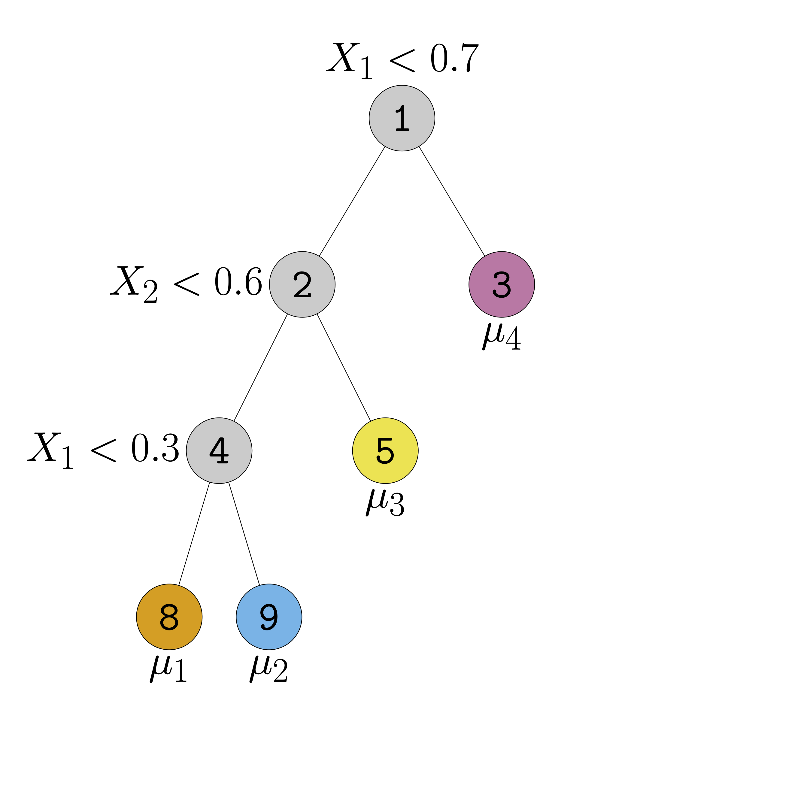
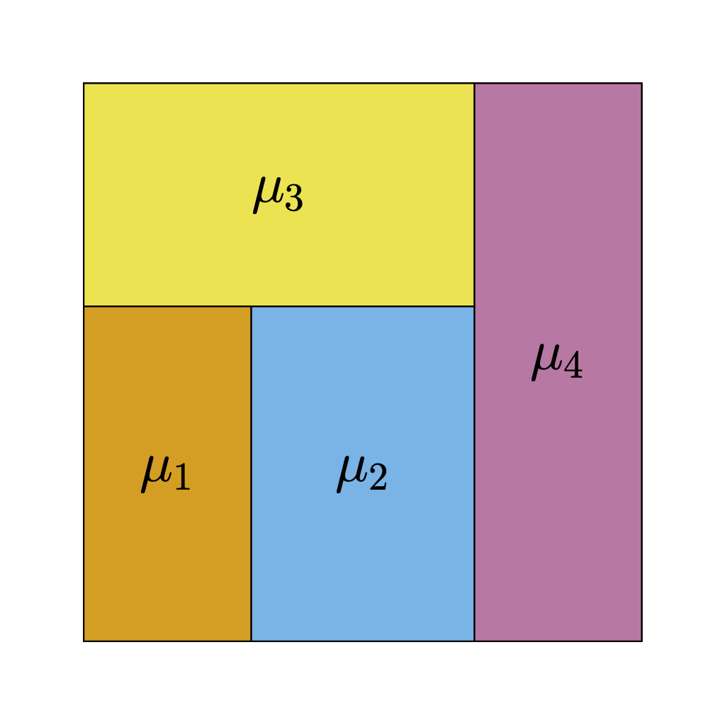
Figure 1 (a) shows an example of a regression tree defined over the space \([0,1]^{2}\). Regression trees represent piece-wise constant step-functions (Figure 1 (b)). To see this, imagine taking a point \(\boldsymbol{\mathbf{x}} = (x_{1}, \ldots, x_{p})\) and tracing a path from the root of the tree — that is, the node at the very top — down to one of the terminal leaf nodes by following the decision rules. Specifically, when the path encounters an interior node associated with the rule \(\{X_{j} < c\}\), the path proceeds to the left child if \(x_{j} < c\) and the right child otherwise. When the path reaches a leaf \(\ell\), we output the associated scalar \(\mu_{\ell}.\) For instance, in the case of Figure 1 (b), the path associated with every point in the yellow rectangle terminates in the yellow leaf node in Figure 1 (a).
(a) Regression tree
(b) Step function represented by the tree
Figure 1: Regression trees are piecewise-constant step-functions
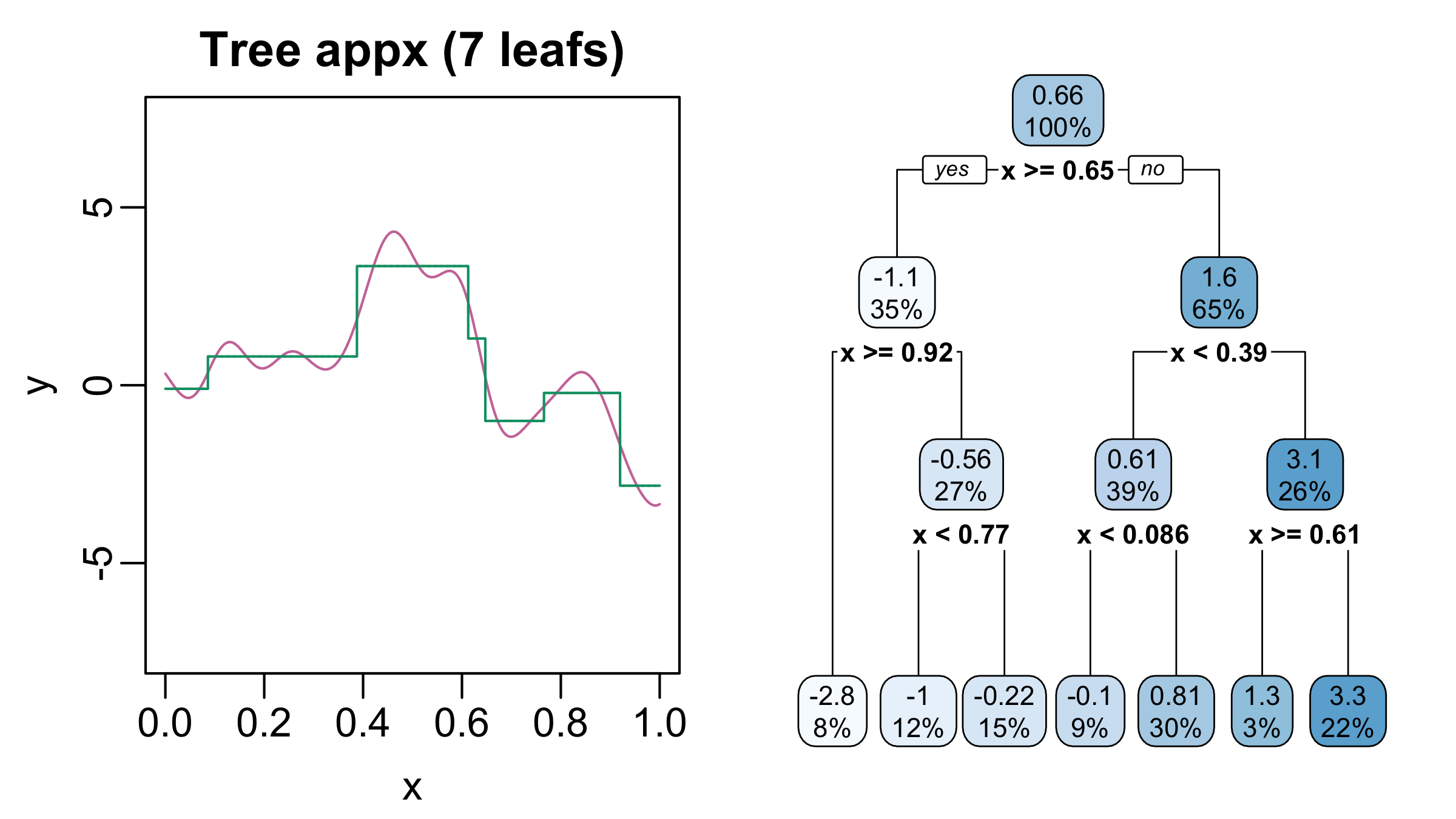
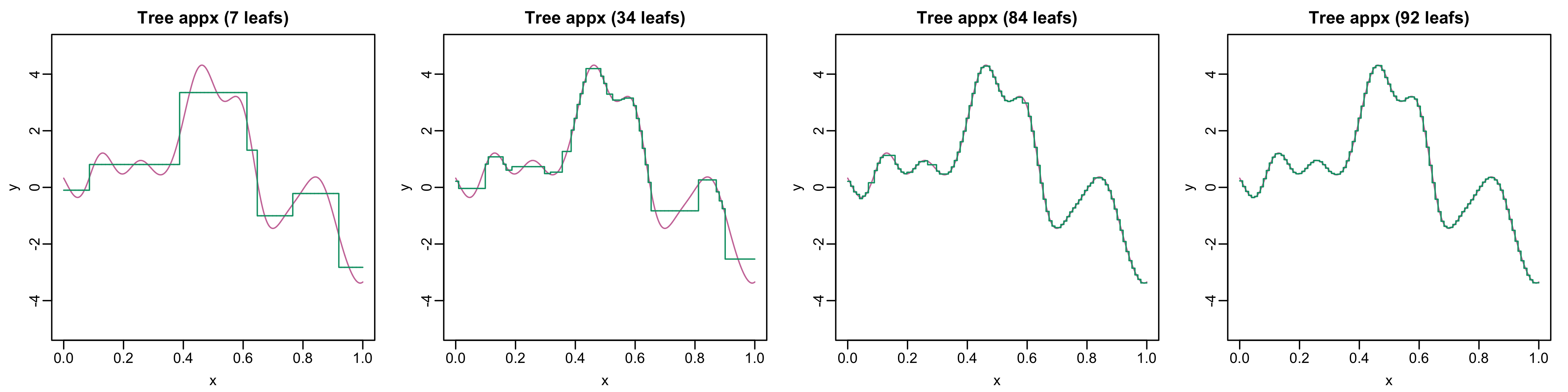
It turns out that regression trees are universal function approximators: for just about every function with \(p\) inputs, there is a regression tree that can approximate the function to an arbitrarily small tolerance. The catch is one often needs a very deep tree, with lots of splits and leaf nodes to obtain a highly accurate approximation. Figure 2 and Figure 3 illustrate this phenomenon. The tree on the right-hand side of Figure 2 has seven leaves and encodes a step function (green curve on the left) Although this step function captures certain macro trends (e.g., the increase around \(x = 0.4\) and subsequent decrease around \(x = 0.6\)) of the true function (pink), it misses a lot of local structure (e.g., the local optima between \(x = 0.2\) and \(x = 0.4\)). But, as the tree gets deeper and number of leaves increases, the approximation improves (Figure 3).
Figure 2: Left: True function (pink) and a step function approximation (green). Right: representation of the step function as a regression tree
Figure 3: As the number of leaves increases (i.e., tree becomes deeper), we obtain more accurate approximations
So, at least conceptually, this makes regression trees a very powerful tool in Statistics: rather than trying to pre-specify the functional form of \(\mathbb{E}[Y \vert \boldsymbol{\mathbf{X}} = \boldsymbol{\mathbf{x}}]\) — that is, manually specifying non-linearities or high-order interactions in a (generalized) linear model — we can instead focus on learning a regression trees5 that fits the data well.
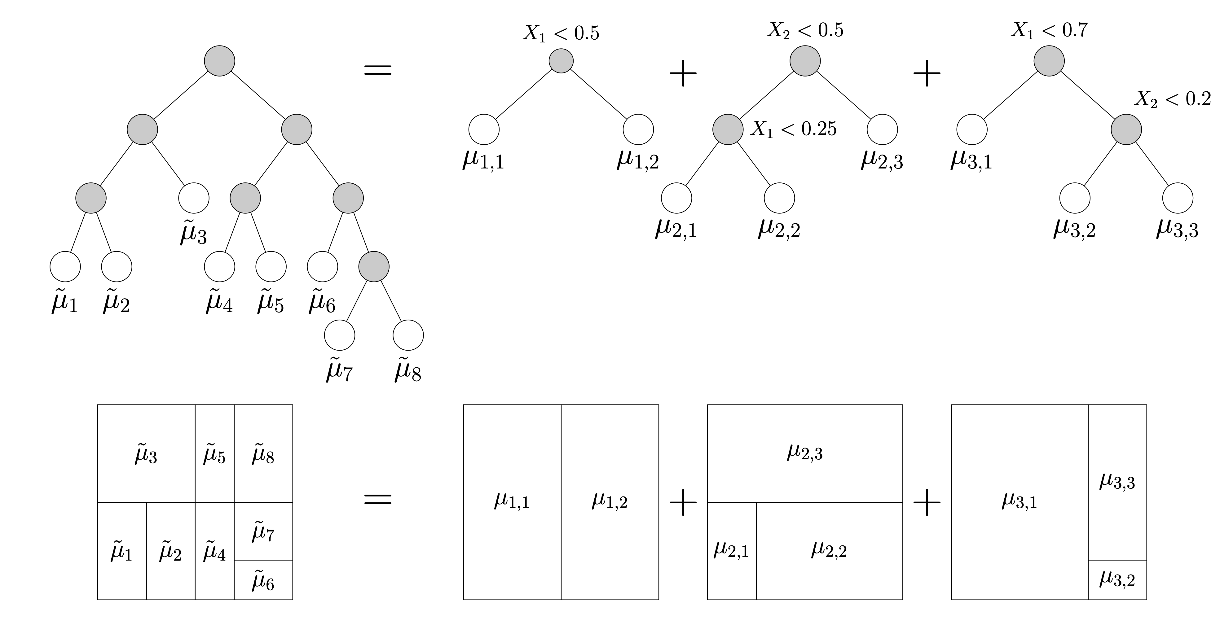
As suggested by Figure 3, we often need a very deep tree with lots of leaves to get a good approximation. Luckily, it turns out that very complicated trees can be decomposed into sums of simpler trees. In Figure 4, we write the somewhat complex tree on the left as a sum of three simpler trees on the right6. We typically refer to a collection of simple regression trees as an ensemble. Methods that make predictions using ensembles of regression trees often out-perform more complicated deep-learning and neural-network models7
Figure 4: Complex trees can be represented as sums of simpler trees
Fitting Random Forests Models
Breiman (2001) introduced the random forests algorithm for estimating a collection of regression trees that, when added up, provided a good approximation to an unknown regression function8. The technical details of this algorithm are beyond the score of this course9
In this course, we will fit random forests models using the ranger package. The main function of that package is called ranger(). Its syntax is somewhat similar to glm() insofar as both functions require us to specify a formula and pass our data in as a data frame (or tibble). Unlike glm(), which required us to specify the argument family = binomial("logit") to fit binary outcomes, ranger() requires us to specify the argument probability=TRUE. This signals to the function that we want predictions on the probability scale and not the \(\{0,1\}\)-outcome scale.
We can also use predict() to get predictions from a model fitted with ranger(). But this also involves slightly different syntax: instead of using the argument newdata, we need to use the argument data. Additionally, when making predictions based on a ranger model with probability = TRUE, the function predict returns a named list. One element of that list is called predictions and it is a matrix whose rows correspond to the rows of data and whose columns contain the probabilities \(\mathbb{P}(Y = 0)\) and \(\mathbb{P}(Y = 1).\) So, to get the predicting XG values, we need to look at the 2nd column of this matrix.
The . is short-hand for “all of the columns in dataexcept for what’s on the left-hand side of the ~”
2
When making a prediction using the output of ranger, we pass the data in using the data argument instead of newdata.
3
As noted earlier, predict returns a list, one of whose elements is a two-column matrix containing the fitted probability. This matrix is stored in the list element predictions. The second column of this matrix contains the fitted probabilities of a goal (\(Y = 1\)).
[1] 0.1135258
[1] 0.2522654
At least for this training/testing split, our in-sample log-loss is much smaller than our out-of-sample log-loss. This is not at all surprising: flexible regression models like random forests are trained to predict the in-sample data and so we should expect to see smaller training errors than testing errors.
Repeating these calculations over 100 training/testing splits, we can conclude that our more flexible random forest model, which accounts for many more features and can accommodate many more interaction terms than our simple logistic regression model, out-performs the logistic regression models.
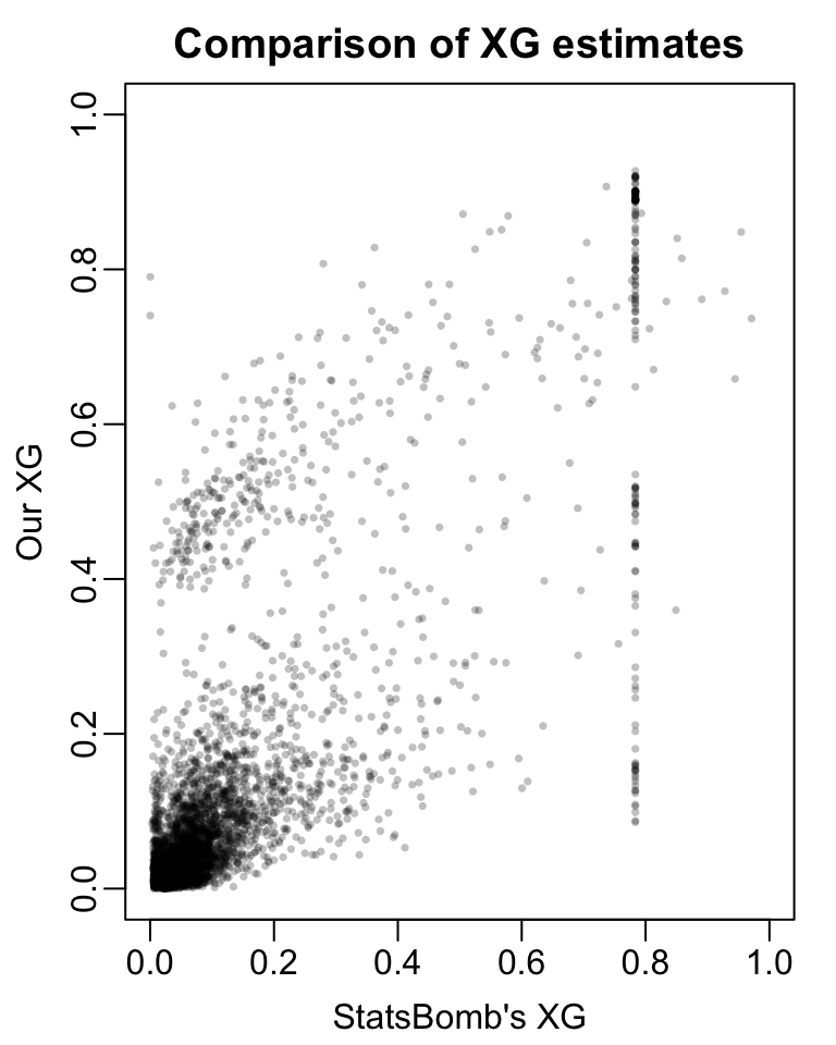
Now that we have a much more predictive model, we can compare our model estimates to those from StatsBomb’s proprietary model. In the code below, we re-fit a random forests model to the whole dataset. We then plot our XG estimates against StatsBomb’s.
full_data <- wi_shots |> dplyr::select(dplyr::all_of(c(shot_vars)))full_rf_fit <- ranger::ranger(formula = Y~.,data = full_data, probability =TRUE)preds <-predict(object = fit, data = full_data)$predictions[,2]par(mar =c(3,3,2,1), mgp =c(1.8, 0.5, 0))plot(wi_shots$shot.statsbomb_xg, preds,pch =16, cex =0.5, col =rgb(0,0,0, 0.25),xlim =c(0, 1), ylim =c(0,1),xlab ="StatsBomb's XG", ylab ="Our XG", main ='Comparison of XG estimates')
Figure 5
If our model perfectly reproduced StatsBomb’s, we would expect to see all the points in the figure line up on the 45-degree diagonal. In fact, we observe some fairly substantial deviations from StatsBomb’s estimates. In particular, there are some shots for which StatsBomb’s model returns an XG of about 0.8. Our random forests model, on the other hand, returns a range of XG values for those shots. We also see that there are some shots for which StatsBomb’s model returns very small XG;s but our model returns XG’s closer to 0.5
Ultimately, the fact that our model estimates do not match StatsBomb’s is not especially concerning. For one thing, we trained our model using only about 3800 shots from women’s international matches contained in the public data. StatsBomb, on the other hand, trained their model using their full corpus of match data.
More substantively, StatsBomb’s model also conditions on many more features than ours. If our model estimates exactly matched StatsBomb’s, that would indicate that these extra features offered no additional predictive value. Considering that StatsBomb’s XG models condition on the height of the ball when the shot was attempted, the differences seem less surprising.
Exercises
Create a new feature ConeAngle that measures the angle formed by connecting the shot location to the goal posts (whose coordinates are (120,36) and c(120,44)). What sort of relationship would you expect between ConeAngle and XG?
Create a new feature ConeArea that measures the area of the triangle formed by connecting the shot location to the goal posts. What sort of relationship would you expect between ConeArea and XG?
Using 100 random training/testing splits, how much more predictive accuracy is gained (if any) by including ConeAngle, ConeArea, and both ConeAngle & ConeArea in our random forests model.
In lecture, we trained our XG models using data only from women’s international competitions. Train an XG model using data from at least 5 different competitions/seasons and assess how similar its predications are to the ones provided by StatsBomb
Grinsztajn, Léo, Edouard Oyallaon, and Gaël Varoquaux. 2022. “Why Do Tree-Based Models Still Outperfom Deep Learning on Tabular Data?”
Footnotes
Our notation nods to the fact that predicted XG is just a predicted probability↩︎
We often convert categorical features like shot.body_part.name or shot.technique.name into several numerical features using one-hot encoding.↩︎
These are known as genearlized linear models and include things like logistic regression and Poisson regression. See Chatper 5 of Beyond Multiple Linear Regression for a nice overview.↩︎
see this issue in the StatsBomb’s opendata GitHub repo for more information about the variable definitions. The code to compute these values is available here. Note that in the StatsBomb coordinate system, the center of the goal line is at (120,4).↩︎
That is, learn the number and arrangement of the interior and leaf nodes as well as the decision rules and leaf outputs↩︎
To verify this decomposition is correct, imagine stacking the three partitions on top of each other.↩︎
The canonical reference is Grinsztajn, Oyallaon, and Varoquaux (2022) (link).↩︎