load("statcast2024.RData")Lecture 11: Pitch Framing
Overview
In October 2015, the Houston Astros played the New York Yankees in the American League Wild Card game. During and after the game, several Yankees fans took to social media to complain about inconsistencies in the strike zone being called by home plate umpire Eric Cooper. They argued that Cooper was not calling balls and strikes consistently for both teams, putting the Yankees at a distinct disadvantage. Beyond simple fan reaction, individual players took exception to Cooper’s strike zone: after striking out, Yankees catcher Brian McCann complained to Cooper that on similar pitches, Cooper was calling strikes when the Astros were pitching but balls when the Yankees were pitching. Figure 1 show two such pitches.
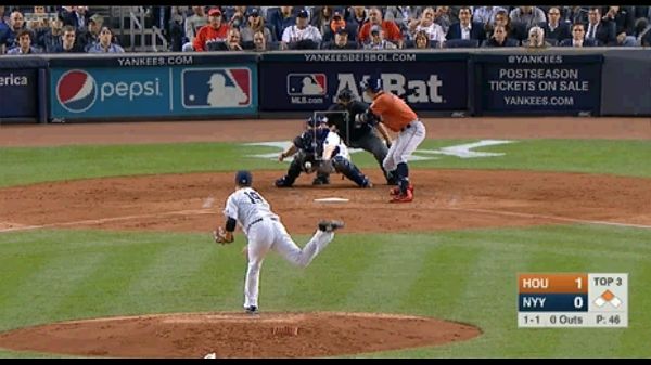
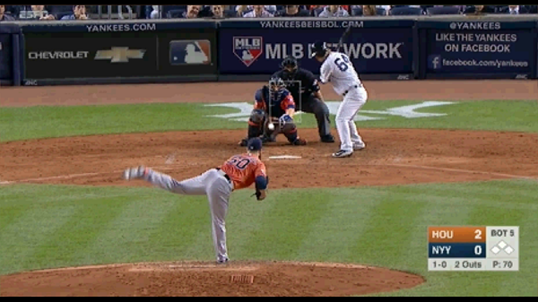
Both pitches were thrown low and outside1, near the bottom left corner of the strike zone2 shown in the figure. Because no part of the ball passed through the strike zone, by rule, both pitches should have been called balls. But umpire Cooper called the pitch in Figure 1 (a), thrown by Yankees pitcher Masahiro Tanaka, a ball and called the pitch in Figure 1 (b), thrown by Astros pitcher Dallas Keuchel, a strike. During the television broadcast of the game and on social media after the game3, many speculated many speculated that the reason for this discrepancy in strike zones is due Astros catcher Jason Castro’s ability to frame pitches, catching them in a way so as to increase the chances of the umpire calling a strike.
Pitch framing, which has been studied by the sabermetrics community since at least 2008, received lots of coverage in the popular press between 2014 and 2016. A good example is this article about Jonathan Lucroy from ESPN The Magazine, which estimated that Lucroy’s framing accounted for a total of two wins for the Brewers in 2014 and was worth around $14 million. That article went on to say that claim that the most impactful player in baseball today is the game’s 17th highest-paid catcher.”
In this lecture, we will estimate how many more runs a catcher saves his team through his framing compared to a replacement-level catcher. Like we did in Lectures 6, 7, and 8, we will work with pitch tracking data scraped from StatCast. We will use the data from 2023 to establish historical strike probabilities (Section 3.1) based on pitch location, batter handedness, and pitcher handedness. We will then include these historical baselines as fixed effects in a multilevel model that also includes random intercepts for the catcher, pitcher, and batter involved in pitches from the 2024 season (Section 3). Using the estimated deviations between catcher intercepts and the grand mean from our multilevel model, we conclude by estimating how many more expected runs catchers save than a replacement-level catcher (Section 4).
Data
Value of a Called Strike
Later, in Section 4, we will compute how many expected runs catchers save their teams To do this, we must first determine the value of a called strike using a similar framework as in Lecture 6. Specifically, we will compute the number of runs scored by the batting the team in the remainder of the half-inning following every pitch. Then, for every combination of the count4 and the number of outs, we will compute the average number of runs scored in the remainder of the half-inning after a called ball and after a called strike on taken pitches5. The difference between these quantities captures the value of a called strike in that particular count-out state.
To compute this, we start by loading the data frame statcast2024 that we prepared and saved in Lecture 6.
Recall that this data table contains a row for every pitch and that the column RunsRemaining recorded how many runs the batting team scored in the remainder of the half-inning following each pitch. We determine whether a pitch was taken using the description field
table(statcast2024$description)
ball_descriptions <-
c("ball", "blocked_ball", "pitchout", "hit_by_pitch")
swing_descriptions <-
c("bunt_foul_tip", "foul", "foul_bunt", "foul_tip",
"hit_into_play", "missed_bunt", "swinging_strike",
"swinging_strike_block")
taken2024 <-
statcast2024 |>
dplyr::filter(!description %in% swing_descriptions) |>
dplyr::mutate(
Y = ifelse(description == "called_strike", 1, 0),
Count = paste(balls, strikes, sep = "-")) |>
dplyr::select(Y, plate_x, plate_z,
Count, Outs,
batter, pitcher, fielder_2,
stand, p_throws,
RunsRemaining, sz_top, sz_bot) |>
dplyr::mutate(
Count = factor(Count),
batter = factor(batter),
pitcher = factor(pitcher),
fielder_2 = factor(fielder_2),
stand = factor(stand),
p_throws = factor(p_throws))- 1
- Extract only the taken pitches
- 2
-
Add columns recording whether taken pitch was called a strike (
Y = 1) or a ball (Y = 0) and the count. - 3
-
fielder_2contains the MLB Advanced Media ID for the catcher - 4
-
standandp_throwsrecord the handedness of the batter and pitcher.
                   ball            blocked_ball           bunt_foul_tip
                 231032                   14717                      15
          called_strike                    foul               foul_bunt
                 113912                  126012                    1208
               foul_tip            hit_by_pitch           hit_into_play
                   7218                    1979                  121751
            missed_bunt                pitchout         swinging_strike
                    196                      52                   73209
swinging_strike_blocked
                   3834
We can now compute the expected numbers of runs scored after a called ball or strike for every combination of out and count.
er_balls <-
  taken2024 |>
  dplyr::filter(Y == 0) |>
  dplyr::group_by(Count, Outs) |>
  dplyr::summarise(er_ball = mean(RunsRemaining), .groups = 'drop')

er_strikes <-
  taken2024 |>
  dplyr::filter(Y == 1) |>
  dplyr::group_by(Count, Outs) |>
  dplyr::summarise(er_strike = mean(RunsRemaining), .groups = 'drop')

er_taken <-
  er_balls |>
  dplyr::left_join(y = er_strikes, by = c("Count", "Outs")) |>
  dplyr::mutate(value = er_ball - er_strike)

er_taken |> dplyr::slice_head(n=5)
# A tibble: 5 × 5
Count Outs er_ball er_strike value
<fct> <int> <dbl> <dbl> <dbl>
1 0-0 0 0.731 0.605 0.126
2 0-0 1 0.547 0.425 0.122
3 0-0 2 0.283 0.193 0.0902
4 0-1 0 0.660 0.525 0.135
5 0-1 1 0.464 0.365 0.0990Looking at er_taken, we find that batting teams score
- About 0.731 runs following a called ball on a 0-0 pitch with 0 outs
- About 0.605 runs following a called strike on a 0-0 pitch with 0 outs So, if a good pitch framer can get a 0-0 pitch with 0 outs called a strike instead of ball, he saves the fielding team about 0.126 runs, on average. From the standpoint of the fielding team, a called strike is most valuable on a 3-2 pitch with 0 outs (when they can expect to save almost 0.8 runs on average) and least value on a 0-1 pitch with 2 outs (when they can expect to save about 0.068 runs on average).
er_taken |> dplyr::arrange(dplyr::desc(value)) |> dplyr::slice(c(1, dplyr::n()))# A tibble: 2 × 5
Count Outs er_ball er_strike value
<fct> <int> <dbl> <dbl> <dbl>
1 3-2 0 1.12 0.321 0.800
2 0-1 2 0.234 0.166 0.0684So that we can use it later in Section 4, we will append a column to taken2024 containing the value of a called strike (from the fielding team’s perspective).
taken2024 <-
  taken2024 |>
  dplyr::left_join(y = er_taken |> dplyr::select(Count, Outs, value), by = c("Count", "Outs"))
A Multilevel Model
We are ultimately interested in understanding how individual players (i.e., batters, catchers, and pitchers) can influence the called strike probability. Any credible model for these probabilities must account for location. After all, if a pitch is thrown several feet away from the batter, no amount of pitch framing will change the call from a ball to a strike. Similarly, catcher skill is likely n The StatCast variables plate_x and plate_z respectively record the horizontal and vertical coordinate of each pitch as it crosses the front edge of home plate. These variables are measured from the catcher’s perspective so pitches thrown to the left of home plate have negative plate_x values and pitches thrown to the right of home plate have positive plate_x values. Both plate_x and plate_z are measured in feet.
A natural starting point is to fit a multilevel model with player-specific random intercepts that adjusts for the fixed effects of plate_x and plate_z. Specifically, because we are dealing with a binary outcome, we might start with the model \[
\log \left( \frac{\mathbb{P}(Y_{i} = 1)}{\mathbb{P}(Y_{i} = 0)} \right) = B_{b[i]} + C_{c[i]} + P_{p[i]} + \beta_{x} x_{i} + \beta_{z}z_{i}
\] where \(b[i], c[i],\) and \(p[i]\) record the identities of the batter, catcher, and pitcher involved in taken pitch \(i;\) \(x_{i}\) and \(z_{i}\) are the plate_x and plate_z measurements; and the \(B_{b}\)’s, \(C_{c}\)’s, and \(P_{p}\)’s are random intercepts for the batters, catchers, and pitchers with \(B_{b} \sim N(\mu_{B}, \sigma^{2}_{B}),\) \(C_{c} \sim N(\mu_{C}, \sigma^{2}_{C})\), and \(P_{p} \sim N(\mu_{P})\). This simple model assumes that the log-odds of a called strike is monotonic in plate_x and plate_z. Due to the monotonicity of the inverse logistic transformation6, a positive (resp. negative) \(\beta_{x}\) would imply that the probability of a called strike increases (resp. decreases) as the pitch moves from left to right. Similarly, a positive (resp. negative) \(\beta_{z}\) implies that the probability of a called strike increases (resp. decreases) the higher up a pitch is thrown.
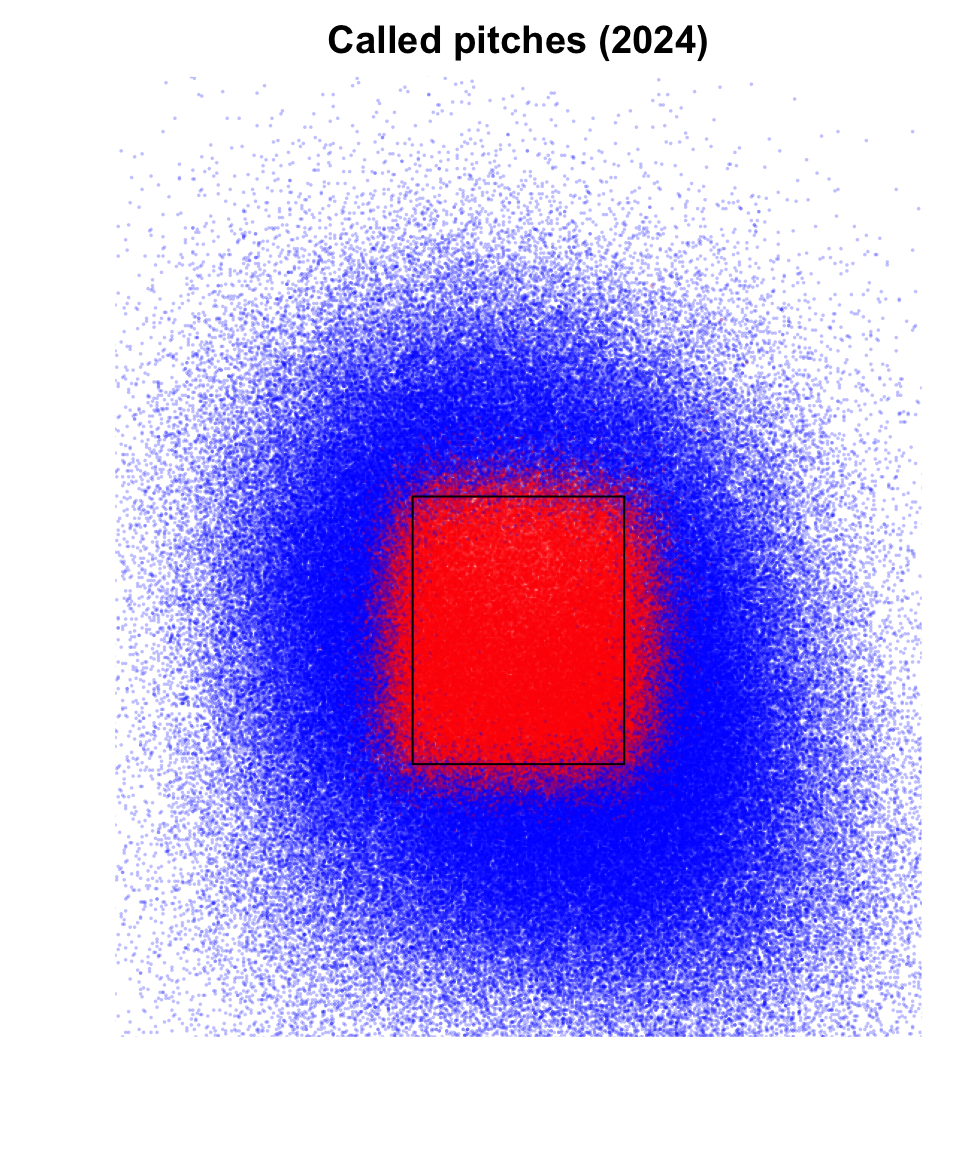
A cursory glance at the data reveals such monotonicity is not realistic. Specifically, if called strike probability was monotonic in plate_x and plate_z, then we should see progressively more strikes in one of the four corners of the plot7. In the plot, we overlay the “average” rule book strike zone8.
par(mar = c(3,3,2,1), mgp = c(1.8, 0.5, 0))
plot(1, type = "n",
xlim = c(-2.5, 2.5), ylim = c(0, 6),
xlab = "", ylab = "",
main = "Called pitches (2024)",
xaxt = "n", yaxt = "n", bty = "n")
points(x = taken2024$plate_x, y = taken2024$plate_z,
pch = 16, cex = 0.25,
col = ifelse(taken2024$Y == 1, rgb(1, 0, 0, 0.25), rgb(0,0,1,0.25)))
rect(xleft = -8.5/12,
ybottom = mean(taken2024$sz_bot, na.rm = TRUE),
xright = 8.5/12,
ytop = mean(taken2024$sz_top, na.rm = TRUE))- 1
-
Restrict attention to pitches that are not in the dirt (i.e.,
plate_z > 0) but not thrown too high (i.e.plate_z < 6), are within 2.5 feet of the center of home plate in either direction. - 2
-
Color strikes (
Y = 1) in red and balls in blue (Y = 0). The 0.25 sets the transparency
Letting \(n_{B}, n_{C},\) and \(n_{P}\) be the numbers of batters, catchers, and pitchers, we will instead model \[ \log \left( \frac{\mathbb{P}(Y_{i} = 1)}{\mathbb{P}(Y_{i} = 0)} \right) = B_{b[i]} + C_{c[i]} + P_{p[i]} + \beta_{p} \log\left(\frac{\hat{p}(x_{i}, z_{i})}{1 - \hat{p}(x_{i}, z_{i})}\right) \] where \(\hat{p}(x,z)\) is a baseline called strike probability estimated using data from the previous season9 and the random player intercepts satisfy \[ \begin{align} B_{b} &= \mu_{B} + u_{b}^{(B)}; \quad u^{(B)}_{b} \sim N(0, \sigma^{2}_{B}) \quad \text{for each}~b = 1, \ldots, n_{B} \\ C_{c} &= \mu_{C} + u_{c}^{(C)}; \quad u^{(C)}_{c} \sim N(0, \sigma^{2}_{C}) \quad \text{for each}~c = 1, \ldots, n_{C} \\ P_{p} &= \mu_{P} + u_{p}^{(P)}; \quad u^{(P)}_{p} \sim N(0, \sigma^{2}_{P}) \quad \text{for each}~p = 1, \ldots, n_{P}. \\ \end{align} \] Our model accounts for pitch location by including a suitably-transformed baseline called strike probability estimate as a fixed effect. The random player intercepts capture how much each player contributions to the log-odds of a called strike over and above what is determined by pitch location.
Historical Strike Probabilities
To fit our proposed multilevel model, we must first compute the baseline called strike probabilities using data from the 2023 season. We first scrape all StatCast data fr om2023 using the function annual_statcast_query, which we defined in Lecture 6 and is available here.
source("annual_statcast_query.R")
raw_statcast2023 <- annual_statcast_query(season = 2023)
save(raw_statcast2023, file = "raw_statcast2023.RData")- 1
- This will only work if the file “annual_statcast_query.R” is saved in your R working directory
We can now apply the same basic pre-processing to raw_statcast2023 that we did to raw_statcast2024 back in Lecture 6.
statcast2023 <-
  raw_statcast2023 |>
  dplyr::filter(game_type == "R") |>
  dplyr::filter(
    strikes >= 0 & strikes < 3 &
      balls >= 0 & balls < 4 &
      outs_when_up >= 0 & outs_when_up < 3) |>
  dplyr::arrange(game_pk, at_bat_number, pitch_number) |>
  dplyr::mutate(
    BaseRunner =
      paste0(1*(!is.na(on_1b)),1*(!is.na(on_2b)),1*(!is.na(on_3b)))) |>
  dplyr::rename(Outs = outs_when_up)
Now that we have pre-processed the 2023 StatCast data, we will extract all called pitches. We will fit our generalized additive model only to pitches with plate_x values between -1.5 and 1.5 and plate_z values between 1 and 6. Beyond this region there are virtually no called strikes. Including pitches that are too far away from the strike zone — i.e., pitches for which the called strike probability is likely exactly zero — can lead to some numerical instabilities when fitting the GAM.
taken2023 <-
  statcast2023 |>
  dplyr::filter(!description %in% swing_descriptions) |>
  dplyr::mutate(
    Y = ifelse(description == "called_strike", 1, 0)) |>
  dplyr::select(Y, plate_x, plate_z, stand, p_throws) |>
  dplyr::filter(!is.na(plate_x) & !is.na(plate_z)) |>
  dplyr::filter(abs(plate_x) <= 1.5 & plate_z >= 1 & plate_z <= 6) |>
  dplyr::mutate(
    stand = factor(stand),
    p_throws = factor(p_throws))
We now fit our generalized additive model.
Warning
The following code takes several minutes to run.
library(mgcv)
hgam_fit <-
bam(formula = Y ~ stand + p_throws + s(plate_x, plate_z),
family = binomial(link="logit"),
data = taken2023)- 1
- The “h” serves as a reminder that we’re getting historical called strike probabilities
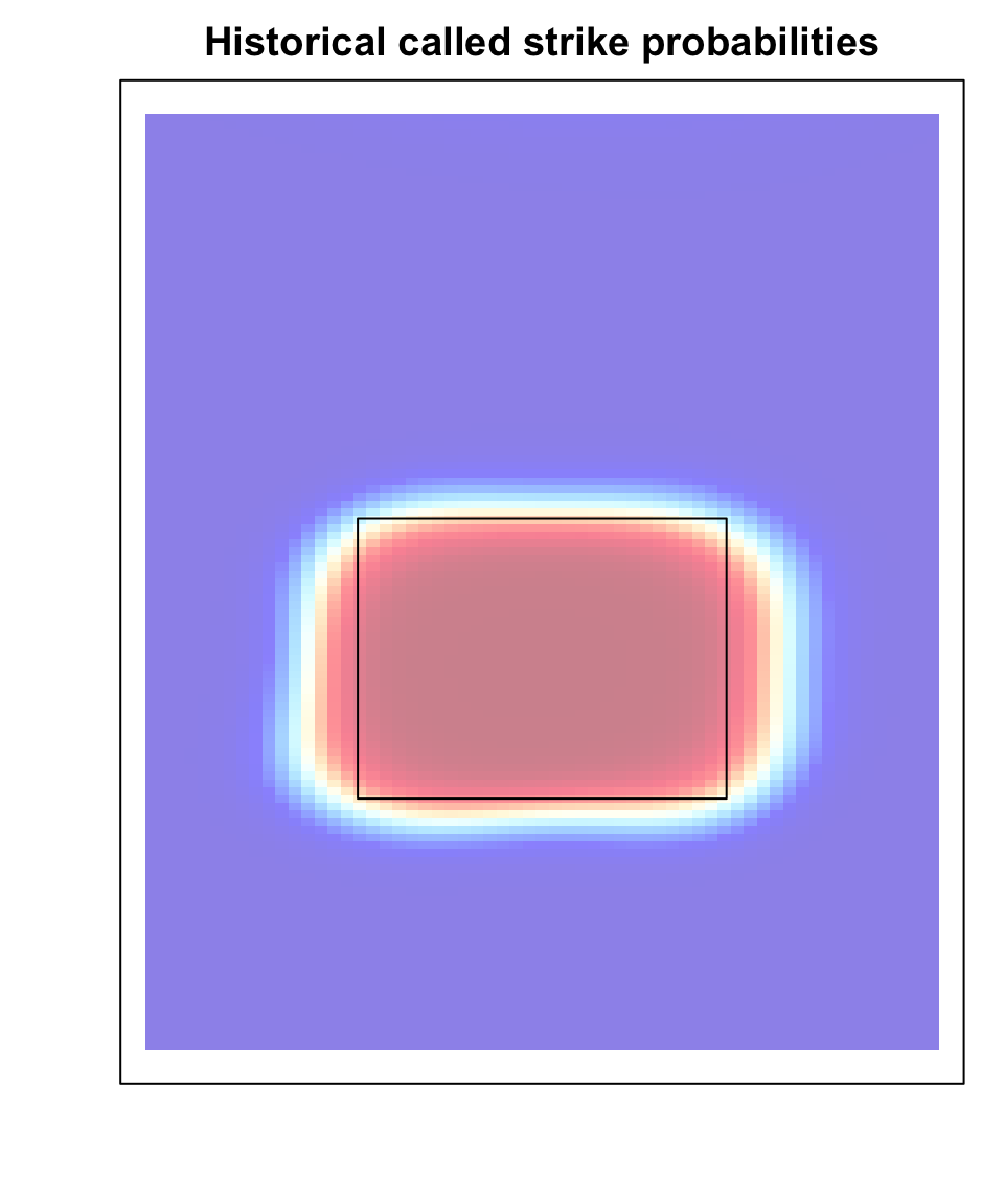
Like we did with our model for the probability of making an out as a function of fielding location in Lecture 8, we can visualize the fitted probabilities along a fine grid of locations. The following code plots the fitted called strike probabilities as a function of location for a right-handed pitcher facing a right-handed batter.
grid_sep <- 0.05
x_grid <- seq(-1.5, 1.5, by = grid_sep)
z_grid <- seq(0, 6, by = grid_sep)
col_list <- colorBlindness::Blue2DarkRed18Steps
plate_grid <-
expand.grid(plate_x = x_grid, plate_z = z_grid) |>
dplyr::mutate(stand = "R", p_throws = "R") |>
dplyr::mutate(stand = factor(stand, levels = c("L", "R")),
p_throws = factor(p_throws, levels = c("L", "R")))
grid_preds <-
predict(object = hgam_fit,
newdata = plate_grid,
type = "response")
grid_prob_cols <-
rgb(colorRamp(col_list,bias=1)(grid_preds)/255)
par(mar = c(3,3,2,1), mgp = c(1.8, 0.5, 0))
plot(1, type = "n",
xlim = c(-1.5, 1.5), ylim = c(0,6),
main = "Historical called strike probabilities",
xlab = "", ylab = "",
xaxt = "n", yaxt = "n")
for(i in 1:nrow(plate_grid)){
rect(xleft = plate_grid$plate_x[i] - grid_sep/2,
ybot = plate_grid$plate_z[i] - grid_sep/2,
xright = plate_grid$plate_x[i] + grid_sep/2,
ytop = plate_grid$plate_z[i] + grid_sep/2,
col = adjustcolor(grid_prob_cols[i], alpha.f = 0.5),
border = NA)
}
rect(xleft = -8.5/12,
ybottom = mean(taken2024$sz_bot, na.rm = TRUE),
xright = 8.5/12,
ytop = mean(taken2024$sz_top, na.rm = TRUE))- 1
- Change this line to visualize the fitted probabilities for different combinations of batter and pitcher handedness
- 2
-
We will eventually pass
plate_gridto thepredictfunction, which will expect bothstandandp_throwsto be factor variables
Fitting Our Multilevel Model
Now that we have fit a GAM model to the historical data, we are ready to compute the baseline log-odds for a called strike for each pitch from 2024. We can do this using the predict function with the argument type = "link" instead of type = "response".
baseline <-
predict(object = hgam_fit,
newdata = taken2024,
type = "link")
taken2024 <-
taken2024 |>
dplyr::mutate(baseline = baseline) |>
dplyr::filter(abs(plate_x) <= 1.5 & plate_z >= 1 & plate_z <= 6)- 1
- We focus only on “frameable” pitches which are not throw too far away from home plate in the horizontal direction and are not thrown too high or too low in the vertical direction.
We’re finally ready to fit our multilevel model
library(lme4)
multilevel_fit <-
glmer(formula = Y ~ 1 + (1 | fielder_2) + (1 | batter) + (1 | pitcher) + baseline,
family = binomial(link = "logit"),
data = taken2024)- 1
-
Because the outcome is binary, we need to use the function
glmer()instead oflmer(). We moreover need to specify thefamilyargument.
Although we cannot estimate the actual player-specific random intercepts \(B_{b}, C_{c}\) and \(P_{p},\) we can estimate the deviations between these the overall global means \(\mu_{B}, \mu_{C},\) and \(\mu_{P}.\) The following code pulls out the deviations for the catchers (i.e., the deviations \(u_{c}^{(C)}\)) and appends these values to
tmp <- ranef(multilevel_fit)
catcher_u <-
data.frame(
fielder_2 = as.integer(rownames(tmp[["fielder_2"]])),
catcher_u = tmp[["fielder_2"]][,1])- 1
-
The MLB Advanced Media IDs are saved as integers but
rownames()returns them as a string.
Runs Saved Above Replacement
The data table catcher_u estimates of the amount each catcher adds to log-odds of a called strike, after adjusting for the historical baseline and the other players, relative to a global average across a super-population of catchers. As we argued in Lecture 10, it is arguably more useful to compare each individual catcher’s performance to a well-defined replacement level rather than to a nebulously defined global average. Noting that most MLB teams carry two catchers on their active roster, we will sort catchers based on the total number of pitches received in the 2024 season. We define the top-60 as non-replacement level and the remaining catchers as replacement-level.
The following code determines the pitch count threshold for defining replacement-level. It then computes the average of the estimated deviations \(u^{(C)}_{c}\)’s across all replacement-level catchers. We will denote this average by \(\overline{u}^{(C)}_{R}.\)
catcher_counts <-
  statcast2024 |>
  dplyr::group_by(fielder_2) |>
  dplyr::summarise(count = dplyr::n()) |>
  dplyr::arrange(dplyr::desc(count))

catcher_threshold <-
  catcher_counts |>
  dplyr::slice(60) |>
  dplyr::pull(count)

catcher_u <-
  catcher_u |>
  dplyr::left_join(y = catcher_counts, by = "fielder_2")

repl_u <-
  catcher_u |>
  dplyr::filter(count < catcher_threshold) |>
  dplyr::pull(catcher_u) |>
  mean()
For every pitch thrown in 2024, we can estimate how the called strike probability changes when the original catcher is replaced with a replacement-level catcher. First, observe that the log-odds of a called strike on pitch \(i\) is given by \[
\mu_{C} + u_{c[i]}^{(C)} + B_{b[i]} + P_{p[i]} + \hat{\beta}_{p} \times \log\left(\frac{\hat{p}(x_{i}, z_{i})}{1 - \hat{p}(x_{i}, z_{i})} \right)
\] We can compute these predicted log-odds using the predict() function and append them to the data table taken2024:
ml_preds <-
predict(object = multilevel_fit,
newdata = taken2024,
type = "link")
taken2024 <-
taken2024 |>
dplyr::mutate(fitted_log_odds = ml_preds)- 1
-
Since we want the fitted log-odds and not the fitted probabilities, we specify
type = "link".
If we replace the original catcher \(c[i]\) with a replacement-level catcher, then the log-odds of a called strike is now \[
\mu_{C} + \overline{u}_{R}^{(C)} + B_{b[i]} + P_{p[i]} + \hat{\beta}_{p} \times \log\left(\frac{\hat{p}(x_{i}, z_{i})}{1 - \hat{p}(x_{i}, z_{i})} \right)
\] To compute the counter-factual log-odds, we need to take the fitted log-odds, subtract the original catcher’s deviation \(u_{c[i]}^{(C)}\), and add the average deviation across all replacement-level catchers (i.e., \(\overline{u}_{R}^{(C)}\)). The following code does this by first appending the estimated \(u^{(C)}_{c[i]}\) to each row of taken2024 and then computing the counter-factual log-odds
taken2024 <-
taken2024 |>
dplyr::left_join(y = catcher_u |>
dplyr::select(fielder_2, catcher_u) |>
dplyr::mutate(fielder_2 = factor(fielder_2)),
by = "fielder_2") |>
dplyr::mutate(repl_log_odds = fitted_log_odds - catcher_u + repl_u) - 1
-
fielder_2is a factor variable intaken2024but a numeric variable incatcher_u. By converting it to a factor, we ensure that the join is successful
The number of expected runs a catcher saves through his framing relative to a replacement-level catcher is the product of the value of a called strike multiplied by the actual and counter-factual called strike probability.
taken2024 <-
  taken2024 |>
  dplyr::mutate(
    fitted_prob = 1/(1 + exp(-1 * fitted_log_odds)),
    repl_prob = 1/(1 + exp(-1 * repl_log_odds)),
    rsar = value * (fitted_prob - repl_prob))
Summing over all pitches received by a catcher over the season, we can compute his total number of runs saved above replacement. In the following code, we load in the player look-up table we created in Lecture 6
load("player2024_lookup.RData")

rsar <-
  taken2024 |>
  dplyr::group_by(fielder_2) |>
  dplyr::summarise(rsar = sum(rsar), n = dplyr::n()) |>
  dplyr::rename(key_mlbam = fielder_2) |>
  dplyr::left_join(player2024_lookup |>
                     dplyr::select(key_mlbam, Name) |>
                     dplyr::mutate(key_mlbam = factor(key_mlbam)), by = "key_mlbam")
There is considerable overlap between the top-10 catchers according to our framing runs saved above replacement metric and the top-10 catchers according to rankings produced by Baseball Savant. Both models, for instance, identify Patrick Bailey, who won a Golden Glove award in 2024, as a particularly strong framer.
rsar |>
  dplyr::arrange(dplyr::desc(rsar)) |>
  dplyr::slice_head(n = 10) |>
  dplyr::select(Name, rsar, n)
# A tibble: 10 × 3
Name rsar n
<chr> <dbl> <int>
1 Patrick Bailey 30.1 6118
2 Cal Raleigh 19.9 6449
3 Austin Wells 17.9 5540
4 Alejandro Kirk 17.3 4761
5 Jake Rogers 16.7 4417
6 Christian Vazquez 15.2 4541
7 Jose Trevino 14.6 3639
8 Francisco Alvarez 13.6 4629
9 Bo Naylor 11.6 5639
10 Yasmani Grandal 11.0 3535References
Deshpande, Sameer K., and Abraham J. Wyner. 2017. “A Hierarchical Bayesian Model of Pitch Framing.” Journal of Quantitative Analysis in Sports 13 (3): 95–12. https://doi.org/10.1515/jqas-2017-0027.
Footnotes
That is, away from the batter.↩︎
The strike zone is defined as “the area over home plate from the midpoint between a batter’s shoulders and the top of the uniform pants – when the batter is in his stance and prepared to swing at a pitched ball – and a point just below the kneecap.” See here.↩︎
See this blogpost for a compilation of posts.↩︎
The numbers of balls and strikes previously called in the at-bat.↩︎
These are pitches in which the batter doesn’t swing.↩︎
If \(u = \log{\frac{p}{1-p}}\) for some \(p \in [0,1],\) then \(p = 1/[1 + e^{-u}]\), which is monotonically increasing as↩︎
Try to prove yourself by considering four cases, one for each combination of the sign of \(\beta_{x}\) and \(\beta_{z}\) in the model above.↩︎
Home plate measures 17 inches across, so we set the horizontal limits at -8.5/12 and 8.5/12. To set the vertical limits, we take the average values of the StatCast variable
sz_topandsz_bot, which are manually determined by the StatCast operator on every pitch↩︎The strategy to include a suitably-transformed baseline probability estimates was first used by Judge, Pavlidis, and Brooks in a 2015 Baseball Prospectus article. It was also used by Deshpande and Wyner (2017) (see Section 2.2 of that paper).↩︎