[1] 0.6224593[1] 0.549834[1] 0.3775407Bradley-Terry Models I
\[ \mathbb{P}(\textrm{WIS beats OSU}) = \textrm{???} \]
Suppose there are \(n\) games played between \(p\) teams
For each team \(j\), there is a latent strength \(\lambda_{j}\) \[ \mathbb{P}(\textrm{team i beats team j}) = \frac{e^{\lambda_{i}}}{e^{\lambda_{i}} + e^{\lambda_{j}}} = \frac{1}{1 + e^{-1 \times (\lambda_{i} - \lambda_{j})}} \]
Log-odds of \(i\) beating \(j\): \(\lambda_{i} - \lambda_{j}.\)
Consider tournament w/ 4 teams and \(\lambda_{1} = 1, \lambda_{2} = 0.5, \lambda_{3} = 0.3\) and \(\lambda_{4} = 0.\)
What is prob. that Team 3 finishes in top-2 in terms of wins?
Enumerate all pairwise probabilities
design <-
  combn(x = 1:4, m = 2) |>
  t() |>
  as.data.frame() |>
  dplyr::rename(player1 = V1, player2 = V2) |>
  dplyr::rowwise() |>
  dplyr::mutate(prob = probs[player1, player2]) |>
  dplyr::ungroup()
design
# A tibble: 6 × 3
player1 player2 prob
<int> <int> <dbl>
1 1 2 0.622
2 1 3 0.668
3 1 4 0.731
4 2 3 0.550
5 2 4 0.622
6 3 4 0.574player1 wins; Tails: player2 winsrbinom(n, size, prob): simulate from a Binomial distributionsize = 1
n: number of coins to flipprob: prob. of each coin landing headstmp_df <-
design |>
dplyr::select(player1, player2) |>
dplyr::mutate(
outcome = outcomes,
winner = ifelse(outcome == 1, player1, player2),
player1 = factor(player1, levels = 1:4),
player2 = factor(player2, levels = 1:4),
winner = factor(winner, levels = 1:4))
tmp_df# A tibble: 6 × 4
player1 player2 outcome winner
<fct> <fct> <int> <fct>
1 1 2 0 2
2 1 3 1 1
3 1 4 1 1
4 2 3 0 3
5 2 4 1 2
6 3 4 1 3 winner & counting occurrencescomplete: fills in missing combinationsn_sims <- 5000
simulated_wins <- matrix(data = NA, nrow = n_sims, ncol = 4)
for(r in 1:n_sims){
set.seed(479+r)
outcomes <- rbinom(n = 6, size = 1, prob = design$prob)
wins <-
design |>
dplyr::select(player1, player2) |>
dplyr::mutate(
outcome = outcomes,
winner = ifelse(outcome == 1, player1, player2),
winner = factor(winner, levels = unique(c(design$player1, design$player2)))) |>
dplyr::group_by(winner) |>
dplyr::summarise(Wins = dplyr::n()) |>
dplyr::rename(Team = winner) |>
tidyr::complete(Team, fill = list(Wins = 0))
simulated_wins[r,] <- wins |> dplyr::pull(Wins)
} [,1] [,2] [,3] [,4]
[1,] 3 1 1 1
[2,] 2 1 1 2
[3,] 2 1 2 1
[4,] 3 2 1 0
[5,] 1 1 3 1
[6,] 3 2 1 0
[7,] 3 1 1 1
[8,] 1 3 1 1
[9,] 1 0 3 2
[10,] 2 3 0 1# A tibble: 10 × 10
Day Date Time Opponent OppScore Home HomeScore OT Notes Type
<chr> <chr> <chr> <chr> <int> <chr> <int> <chr> <chr> <chr>
1 Sat. 1/4/2025 1:00 CT Minneso… 4 Lind… 1 <NA> <NA> NC
2 Fri. 12/6/2024 6:00 ET Connect… 2 New … 1 <NA> <NA> HE
3 Fri. 12/6/2024 6:00 ET Dartmou… 3 Clar… 5 <NA> <NA> EC
4 Fri. 11/29/2024 6:00 ET Colgate 3 Syra… 1 <NA> <NA> NC
5 Sat. 1/18/2025 3:00 ET Renssel… 0 Dart… 0 OT DAR … EC
6 Sat. 3/1/2025 4:30 ET Maine 3 Bost… 4 <NA> HEA … NC
7 Fri. 1/3/2025 7:00 ET Yale 8 Robe… 1 <NA> <NA> NC
8 Fri. 11/1/2024 3:00 CT Minneso… 2 Bemi… 1 <NA> <NA> WC
9 Fri. 1/10/2025 6:00 ET St. Law… 4 Union 2 <NA> <NA> EC
10 Sat. 11/16/2024 12:00 ET Vermont 0 Prov… 0 OT VER … HE HomeScore differs from OppScoreHomeScore==OppScore, game decided in shoot outNotes column# A tibble: 5 × 4
home.team away.team home.win away.win
<fct> <fct> <dbl> <dbl>
1 Wisconsin St. Cloud State 2 0
2 Wisconsin St. Thomas 2 0
3 Wisconsin Minnesota 3 0
4 Wisconsin Ohio State 1 1
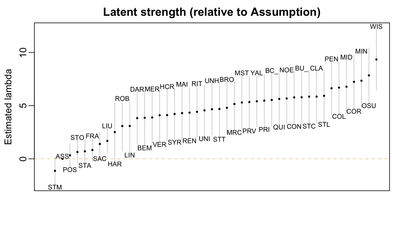
5 Wisconsin Lindenwood 2 0BTm allows us to manually specify reference team (w/ \(\lambda_{j} = 0\))
Call:
BradleyTerry2::BTm(outcome = cbind(home.win, away.win), player1 = home.team,
    player2 = away.team, refcat = "Assumption", data = results)

Coefficients:
                    Estimate Std. Error z value Pr(>|z|)
..Bemidji State       3.8615     1.2828   3.010 0.002610 **
..Boston College      5.5371     1.2307   4.499 6.82e-06 ***
..Boston University   5.7866     1.2267   4.717 2.39e-06 ***
..Brown               4.7983     1.2178   3.940 8.14e-05 ***
..Clarkson            5.8522     1.2137   4.822 1.42e-06 ***
..Colgate             6.6950     1.2248   5.466 4.59e-08 ***
..Connecticut         5.7772     1.2293   4.700 2.61e-06 ***
..Cornell             7.2421     1.2586   5.754 8.72e-09 ***
..Dartmouth           3.8239     1.2433   3.076 0.002100 **
..Franklin Pierce     0.8259     0.5436   1.519 0.128701
..Harvard             2.5128     1.3690   1.835 0.066441 .
..Holy Cross          4.1094     1.2214   3.364 0.000767 ***
..Lindenwood          3.0888     1.2317   2.508 0.012150 *
..LIU                 1.6854     0.5869   2.872 0.004085 **
..Maine               4.2996     1.2360   3.479 0.000504 ***
..Mercyhurst          5.1540     1.2094   4.262 2.03e-05 ***
..Merrimack           3.8888     1.2264   3.171 0.001520 **
..Minnesota           7.3462     1.2685   5.791 6.98e-09 ***
..Minnesota Duluth    6.7823     1.2722   5.331 9.75e-08 ***
..Minnesota State     5.2957     1.2725   4.162 3.16e-05 ***
..New Hampshire       4.6625     1.2191   3.824 0.000131 ***
..Northeastern        5.6740     1.2210   4.647 3.37e-06 ***
..Ohio State          7.8472     1.2946   6.061 1.35e-09 ***
..Penn State          6.6326     1.2569   5.277 1.31e-07 ***
..Post                0.3263     0.5404   0.604 0.545921
..Princeton           5.4717     1.2229   4.474 7.66e-06 ***
..Providence          5.3356     1.2281   4.345 1.40e-05 ***
..Quinnipiac          5.6338     1.2010   4.691 2.72e-06 ***
..Rensselaer          4.3425     1.1913   3.645 0.000267 ***
..RIT                 4.4201     1.2043   3.670 0.000242 ***
..Robert Morris       3.0838     1.1764   2.621 0.008755 **
..Sacred Heart        1.3976     0.5531   2.527 0.011504 *
..St. Anselm          0.7039     0.5387   1.307 0.191287
..St. Cloud State     5.8507     1.2647   4.626 3.73e-06 ***
..St. Lawrence        5.9259     1.2094   4.900 9.58e-07 ***
..St. Michael's      -1.1317     0.6421  -1.762 0.077987 .
..St. Thomas          4.6868     1.2861   3.644 0.000268 ***
..Stonehill           0.6387     0.5612   1.138 0.255106
..Syracuse            4.2144     1.1961   3.523 0.000426 ***
..Union               4.5583     1.2002   3.798 0.000146 ***
..Vermont             4.0937     1.2304   3.327 0.000877 ***
..Wisconsin           9.3418     1.4304   6.531 6.53e-11 ***
..Yale                5.4095     1.2138   4.457 8.32e-06 ***
---
Signif. codes:  0 '***' 0.001 '**' 0.01 '*' 0.05 '.' 0.1 ' ' 1

(Dispersion parameter for binomial family taken to be 1)

    Null deviance: 815.15  on 474  degrees of freedom
Residual deviance: 463.44  on 431  degrees of freedom
AIC: 668.78
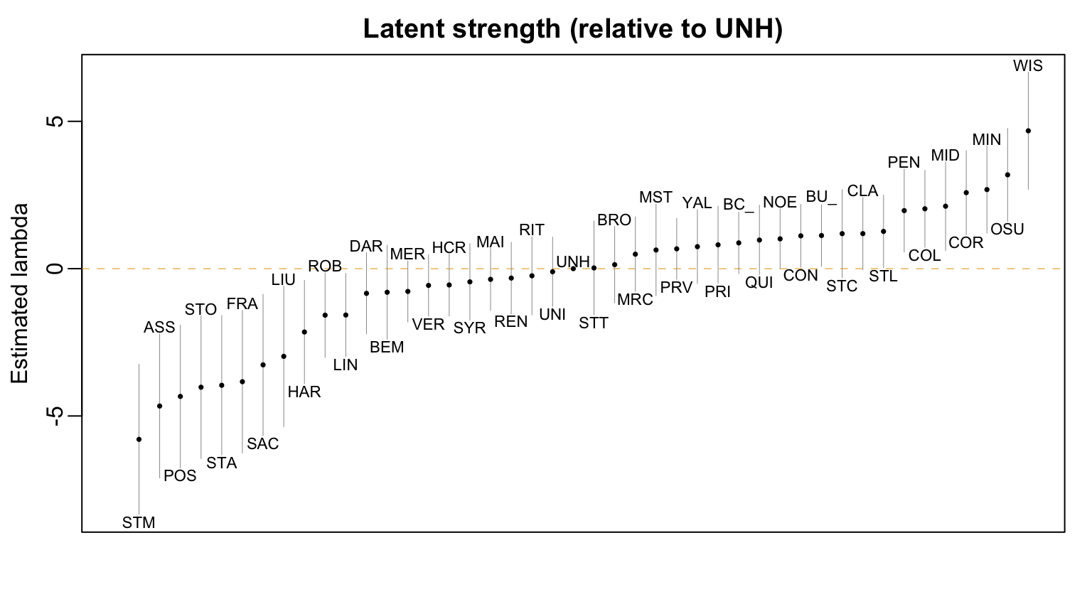
Number of Fisher Scoring iterations: 6BTabilities to extract estimates & standard errorsfit_nh <- update(fit, refcat = "New Hampshire")
lambda_hat_nh <- BradleyTerry2::BTabilities(fit_nh)
lambda_hat_nh[c("Assumption", "New Hampshire", "Wisconsin", "Ohio State"),] ability s.e.
Assumption -4.662547 1.2191462
New Hampshire 0.000000 0.0000000
Wisconsin 4.679297 0.9932217
Ohio State 3.184629 0.7887300[1] 0.8167779wi_wins <- 0
osu_wins <- 0
wi_prob <-
1/(1 + exp(-1 * (lambda_hat["Wisconsin", "ability"] - lambda_hat["Ohio State", "ability"])))
game_counter <- 0
outcomes <- rep(NA, times= 5)
set.seed(481)
while( wi_wins < 3 & osu_wins < 3 & game_counter < 5){
game_counter <- game_counter + 1
outcomes[game_counter] <- rbinom(n = 1, size = 1, prob = wi_prob)
if(outcomes[game_counter] == 1) wi_wins <- wi_wins + 1
else if(outcomes[game_counter] == 0) osu_wins <- osu_wins + 1
}
if(wi_wins == 3){
winner <- "Wisconsin"
} else if(osu_wins == 3){
winner <- "Ohio State"
} else{
winner <- NA
}
cat("Series ended after", game_counter, " games. Winner = ", winner, "\n")
cat("Wisconsin: ", wi_wins, " Ohio State: ", osu_wins, "\n")
cat("Game results:", outcomes, "\n")Series ended after 4 games. Winner = Wisconsin
Wisconsin: 3 Ohio State: 1
Game results: 1 1 0 1 NA