Probit BART • flexBART

Probit Regression

The probit BART model asserts that $\mathbb{P}(Y = 1) = \Phi( f(\boldsymbol{\mathbf{X}}))$ where $\Phi$ is the cumulative distribution function of the standard normal and approximates the unknown function $f$ with a regression tree ensemble. In the original BART paper, Chipman et al. sampled from the probit BART posterior using a Gibbs sampler based on the standard Albert & Chib (1993) data augmentation strategy. Specifically, they introduce a latent variable $Y^{\star} \sim N(f(\boldsymbol{\mathbf{X}}), 1)$ such that $Y = 1(Y^{\star} > 0).$ They then sampled from the posterior induced by this augmented model using a Gibbs sampler which alternated between drawing new values of the latent $Y^{\star}$ ’s conditionally on the regression trees and updating the regression trees conditionally given the latent variables.

When run with the additional argument family = binomial(link="probit"), the function flexBART() implements this sampler based on data augmentation.

To demonstrate, we will generate observations from a probit BART model where the unknown function $f(\boldsymbol{\mathbf{X}})$ only depends on $X_{1}.$ We construct $f$ using random Fourier features and scale $f$ so that it does not take values outside the range [-2,2].

f_true <- function(df){
  stopifnot(all(abs(df[,1]) <= 1))
  
  set.seed(517)
  D <- 5000
  omega0 <- rnorm(n = D, mean = 0, sd = 1.5)
  b0 <- 2 * pi * runif(n = D, min = 0, max = 1)
  weights <- rnorm(n = D, mean = 0, sd = 2*1/sqrt(D))
  u <- 5*df[,1] # re-scale x1 to [-5,5]
  if(length(u) == 1){
    phi <- sqrt(2) * cos(b0 + omega0*u)
    out <- sum(weights * phi)
  } else{
    phi_mat <- matrix(nrow = length(u), ncol = D)
    for(d in 1:D){
      phi_mat[,d] <- sqrt(2) * cos(b0[d] + omega0[d] * u)
    }
    out <- phi_mat %*% weights
  }
  return(out/2.5)
}

Here is what the function $f(\boldsymbol{\mathbf{X}})$ and the corresponding probability function $\Phi(f(\boldsymbol{\mathbf{X}}))$ look like.

Code


par(mar = c(3,3,2,1), mgp = c(1.8, 0.5, 0), mfrow = c(1,2))
x_grid <- seq(-1, 1, by = 0.01)
f_grid <- f_true(data.frame(X1 = x_grid))
p_grid <- pnorm(f_grid)

plot(1, type = "n", xlim = c(-1,1), ylim = c(-2,2), 
     xlab = "X1", ylab = "f(X)", main = "Probit Scale")
lines(x_grid, f_grid)

plot(1, type = "n", xlim = c(-1,1), ylim = c(0,1),
     xlab = "X1", ylab = "Phi(f(X))", main = "Probability Scale")
lines(x_grid, p_grid)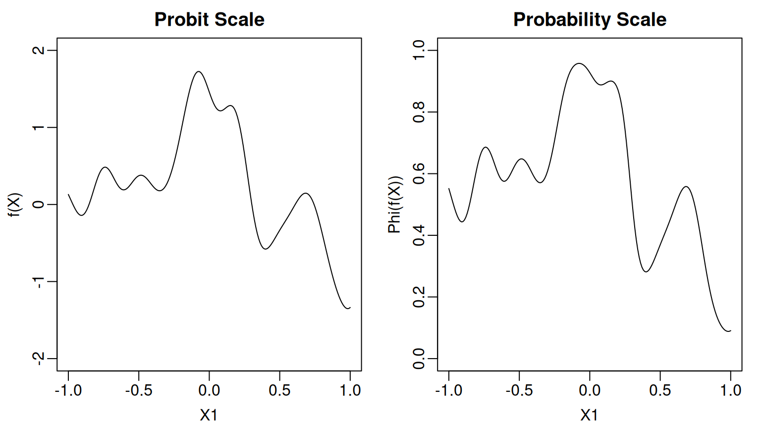

True function on probit (left) probability (right) scale

We generate $n = 5000$ training observations where the first predictor $X_{1}$ is drawn uniformly from the interval $[-1,1].$ We additionally draw nine irrelevant predictors $X_{2}, \ldots, X_{10}$ from the same distribution.

set.seed(105)
n_train <- 5000
p_cont <- 10
train_data <- data.frame(Y = rep(NA, times = n_train))
for(j in 1:p_cont) train_data[[paste0("X", j)]] <- runif(n = n_train, min = -1, max = 1)
f_train <- f_true(train_data[,paste0("X", 1:p_cont)])
prob_train <- pnorm(f_train)

train_data$Y <- rbinom(n = n_train, size = 1, prob = prob_train)

When run with the argument family=binomial(link="probit"), the function flexBART() outputs an object that, like the function pbart() from the BART package, with an attribute prob.train.mean, which contains the posterior means of the $\Phi(f(\boldsymbol{\mathbf{x}}_{i}))$ ’s. When save_samples = TRUE (the default setting), the output also includes the attribute prob.train, which is a matrix containing the posterior samples of the $\Phi(f(\boldsymbol{\mathbf{x}}_{i}))$ values. The rows of prob.trainindex MCMC draws and the columns indexes observations in the training dataset. When used to fit a probit BART model, flexBART() does not return posterior means or samples of the $f(\boldsymbol{\mathbf{x}}_{i})$ ’s, as these can be computed directly from the outputted probabilities.

library(flexBART)
fit <- flexBART(formula = Y ~ bart(.), train_data = train_data,family = binomial(link = "probit"))

The coverage of the pointwise 95% posterior credible intervals for $\Phi(f(\boldsymbol{\mathbf{X}}))$ evaluated at the training observations is higher-than-nominal.

train_quantiles <-
  apply(fit$prob.train, MARGIN = 2, 
        FUN = quantile, 
        probs = c(0.025, 0.975)) |>
  t() |>
  as.data.frame()
mean( prob_train >= train_quantiles[,"2.5%"] & prob_train <= train_quantiles[,"97.5%"])
#> [1] 0.9596

Since the true function $f$ depends only on $X_{1},$ we can visualize the posterior mean and uncertainty intervals as a function of $X_{1}.$ To this end, we create a second data set in which the $X_{1}$ values are evenly spaced between -1 and 1 and the values of the remaining, irrelevant predictors are drawn uniformly from the interval [-1,1]. We then use predict() to draw posterior samples of $\Phi(f(\boldsymbol{\mathbf{X}}))$ evaluated at these new observations. For basic probit BART models, predict() returns a matrix of posterior draws where the rows (resp. columns) index MCMC samples (resp. observations).

x_grid <- seq(-1,1, by = 0.01)
test_data <- data.frame(X1 = x_grid)
for(j in 2:p_cont) test_data[[paste0("X",j)]] <- runif(n = length(x_grid), min = -1, max = 1)
prob_test <- pnorm(f_true(test_data))

pred <- predict(fit, newdata = test_data)

grid_summary <-
  data.frame(
    MEAN = apply(pred, MARGIN = 2, FUN = mean),
    L95 = apply(pred, MARGIN = 2, FUN = quantile, probs = 0.025),
    U95 = apply(pred, MARGIN = 2, FUN = quantile, probs = 0.975))

We see that the posterior mean of $\Phi(f(\boldsybmol{\mathbf{X}}))$ closely tracks the actual function and most of the pointwise 95% credible intervals cover the actual function values

Code

oi_colors <- palette.colors(palette = "Okabe-Ito")
par(mar = c(3,3,2,1), mgp = c(1.8, 0.5, 0))
plot(1, type = "n", xlim = c(-1,1), ylim = c(0,1),
     xlab = "X1", ylab = "Phi(f(X))", main = "P(Y = 1 | X)")
polygon(x = c(x_grid, rev(x_grid)),
        y = c(grid_summary$L95, rev(grid_summary$U95)),
        col = adjustcolor(oi_colors[3], alpha.f = 0.5),
        border = NA)
lines(x_grid, grid_summary$MEAN, col = oi_colors[3])
lines(x_grid, prob_test)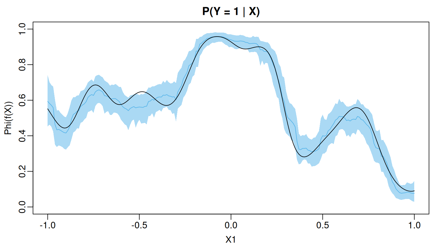

Figure 1: Actual value (black) and posterior mean (blue) of the function $\Phi(f(\boldsymbol{\mathbf{X}}))$ . Pointwise 95% posterior credible intervals are shaded.

At least for these data, the only predictor whose marginal posterior inclusion probability exceeds 50% is $X_{1}.$ The irrelevant predictors $X_{2}, \ldots, X_{9}$ all have inclusion probabilities much less than that.

apply(fit$varcounts >= 1, MARGIN = c(2,3), FUN = mean) |> t()
#>      X1    X2      X3      X4      X5      X6      X7     X8      X9   X10
#> [1,]  1 0.017 0.02125 0.10625 0.01375 0.02475 0.11175 0.0235 0.00675 0.001