Linear Varying Coefficients Model • flexBART

Overview

A linear varying coefficient model posits a linear relationship between an outcome $Y$ and certain covariates $Z_{1}, \ldots, Z_{R}$ but allows that relationship to change with respect to the values of other variables $X_{1}, \ldots, X_{p}.$ That is, a linear varying coefficient model has the form $Y = \beta_{0}(X) + \beta_{1}(X) \times Z_{1} + \cdots + \beta_{R-1}(X) \times Z_{R-1} + \sigma \epsilon,$ where each function $\beta_{r}(X)$ is approximated with an ensemble of regression trees and the error $\epsilon \sim N(0,1).$ Deshpande et al. (2024) introduced VCBART, which extends the basic BART model and estimates each covariate function $\beta_{0}(\boldsymbol{\mathbf{X}}), \ldots, \beta_{R-1}(\boldsymbol{\mathbf{X}})$ with its own regression tree ensemble¹. flexBART supports fitting such VCBART models but provides much more control over the individual ensembles than the original VCBART implementation. Specifically, flexBART allows the size (specified using the optional argument M_vec or M), the tree prior hyperparameters (specified using the optional arguments alpha_vec and beta_vec), and the variables used for splitting (specified via the formula argument) to vary in each ensemble. flexBART also allows different splitting variables to used for each coefficient ensemble.

Example

We first demonstrate flexBART’s functionality using data generated from the model $Y = \beta_{0}(\boldsymbol{\mathbf{X}}) + \beta_{1}(\boldsymbol{\mathbf{X}})Z_{1} + \beta_{2}(\boldsymbol{\mathbf{X}})Z_{2} + \sigma\epsilon,$ where $\boldsymbol{\mathbf{X}}$ contains $p_{\text{cont}} = 10$ continuous and $p_{\text{cat}} = 10$ categorical predictor. Each categorical covariate will take on 10 different values. We will generate $n = 10000$ training observations and $n = 5000$ testing observations.

set.seed(727)
n_train <- 10000
n_test <- 1000
p_cont <- 10
p_cat <- 10
sigma <- 1

We draw each continuous $X_{j}$ uniformly from $[-1,1]$ and each categorical $X_{j}$ uniformly from the set $\{1, 2, \ldots, 10\}.$

train_data <- data.frame(Y = rep(NA, times = n_train))
test_data <- data.frame(Y = rep(NA, times = n_test))
for(j in 1:p_cont){
  train_data[,paste0("X",j)] <- runif(n = n_train, min = -1, max = 1)
  test_data[,paste0("X",j)] <- runif(n = n_test, min = -1, max = 1)
}
for(j in 1:p_cat){
  train_data[,paste0("X",j+p_cont)] <- 
    factor(sample(1:10, size = n_train, replace = TRUE), levels = 1:10)
  test_data[,paste0("X",j+p_cont)] <-
    factor(sample(1:10, size = n_test, replace = TRUE), levels = 1:10)
}

For simplicity, we draw the covariates $Z_{1}$ and $Z_{2}$ from a $N(0,1)$ distribution.

train_data[,"Z1"] <- rnorm(n = n_train, mean = 0, sd = 1)
test_data[,"Z1"] <- rnorm(n = n_test, mean = 0, sd = 1)

train_data[,"Z2"] <- rnorm(n = n_train, mean = 0, sd = 1)
test_data[,"Z2"] <- rnorm(n = n_test, mean = 0, sd = 1)

The three coefficient functions $\beta_{0}(\boldsymbol{\mathbf{X}}), \beta_{1}(\boldsymbol{\mathbf{X}}),$ and $\beta_{2}(\boldsymbol{\mathbf{X}})$ are defined below.

beta0_true <- function(df){
  tmp_X1 <- (1+df[,"X1"])/2 # re-scale X1 to [0,1]
  tmp_X11 <- 1*(df[,"X11"] %in% c(1, 2, 5, 6, 9))
  return(3 * tmp_X1 + (2 - 5 * (tmp_X11)) * sin(pi * tmp_X1) - 2 * (tmp_X11))
}

set.seed(517)
D <- 5000
omega0 <- rnorm(n = D, mean = 0, sd = 1.5)
b0 <- 2 * pi * runif(n = D, min = 0, max = 1)
weights <- rnorm(n = D, mean = 0, sd = 2*1/sqrt(D))
beta1_true <- function(df){
  u <- 5*df[,"X1"] # re-scale x1 to [-5,5]
  if(length(u) == 1){
    phi <- sqrt(2) * cos(b0 + omega0*u)
    out <- sum(weights * phi)
  } else{
    phi_mat <- matrix(nrow = length(u), ncol = D)
    for(d in 1:D){
      phi_mat[,d] <- sqrt(2) * cos(b0[d] + omega0[d] * u)
    }
    out <- phi_mat %*% weights
  }
  return(out)
}

beta2_true <- function(df){
  tmp_X <- (1+df[,"X1"])/2 #re-scale X1 to [0,1]
  return( (3 - 3*cos(6*pi*tmp_X) * tmp_X^2) * (tmp_X > 0.6) - 
    (10 * sqrt(tmp_X)) * (tmp_X < 0.25))
}

We now evaluate the true slopes and response surface function $\mathbb{E}[Y \vert \boldsymbol{\mathbf{X}}, \boldsymbol{\mathbf{Z}}]$ on the training and testing observations

beta0_train <- beta0_true(train_data)
beta0_test <- beta0_true(test_data)

beta1_train <- beta1_true(train_data)
beta1_test <- beta1_true(test_data)

beta2_train <- beta2_true(train_data)
beta2_test <- beta2_true(test_data)

mu_train <-
  beta0_train + train_data[,"Z1"] * beta1_train + train_data[,"Z2"] * beta2_train

mu_test <- 
  beta0_test + test_data[,"Z1"] * beta1_test + test_data[,"Z2"] * beta2_test

train_data[,"Y"] <-
  mu_train + sigma * rnorm(n = n_train, mean = 0, sd = 1)

test_data <- test_data[,colnames(test_data) != "Y"]

Fitting the Model

We’re now ready to fit our model.

set.seed(99)
library(flexBART)
fit <- flexBART(
  formula = Y ~ bart(.) + Z1 * bart(.) + Z2 * bart(.),
  train_data = train_data, test_data = test_data)

flexBART::flexBART returns the posterior mean estimate and posterior samples for each $\beta_{j}(\boldsymbol{\mathbf{x}})$ evaluation (outputs named beta) and for the whole response surface $[Y = , = ] (outputs named yhat). We first plot the posterior mean evaluations of each $\beta_{j}$ and the response surface for both training and testing observations.

Code

# Okabe-Ito colorblind friendly palette
oi_colors <- palette.colors(palette = "Okabe-Ito")

par(mar = c(3,3,2,1), mgp = c(1.8, 0.5, 0), mfrow = c(2,4))
plot(mu_train, fit$yhat.train.mean, pch = 16, cex = 0.5,
     xlab = "Actual", ylab = "Posterior Mean", main = "Response surface (train)")
abline(a = 0, b = 1, col = oi_colors[3])
plot(beta0_train, fit$beta.train.mean[,1], pch = 16, cex = 0.5,
     xlab = "Actual", ylab = "Posterior Mean", main = "Intercept (train)")
abline(a = 0, b = 1, col = oi_colors[3])
plot(beta1_train, fit$beta.train.mean[,2], pch = 16, cex = 0.5,
     xlab = "Actual", ylab = "Posterior Mean", main = "beta1 (train)")
abline(a = 0, b = 1, col = oi_colors[3])
plot(beta2_train, fit$beta.train.mean[,3], pch = 16, cex = 0.5,
     xlab = "Actual", ylab = "Posterior Mean", main = "beta2 (train)")
abline(a = 0, b = 1, col = oi_colors[3])


plot(mu_test, fit$yhat.test.mean, pch = 16, cex = 0.5,
     xlab = "Actual", ylab = "Posterior Mean", main = "Response surface (test)")
abline(a = 0, b = 1, col = oi_colors[3])

plot(beta0_test, fit$beta.test.mean[,1], pch = 16, cex = 0.5,
     xlab = "Actual", ylab = "Posterior Mean", main = "Intercept (test)")
abline(a = 0, b = 1, col = oi_colors[3])

plot(beta1_test, fit$beta.test.mean[,2], pch = 16, cex = 0.5,
     xlab = "Actual", ylab = "Posterior Mean", main = "beta1 (test)")
abline(a = 0, b = 1, col = oi_colors[3])

plot(beta2_test, fit$beta.test.mean[,3], pch = 16, cex = 0.5,
     xlab = "Actual", ylab = "Posterior Mean", main = "beta2 (test)")
abline(a = 0, b = 1, col = oi_colors[3])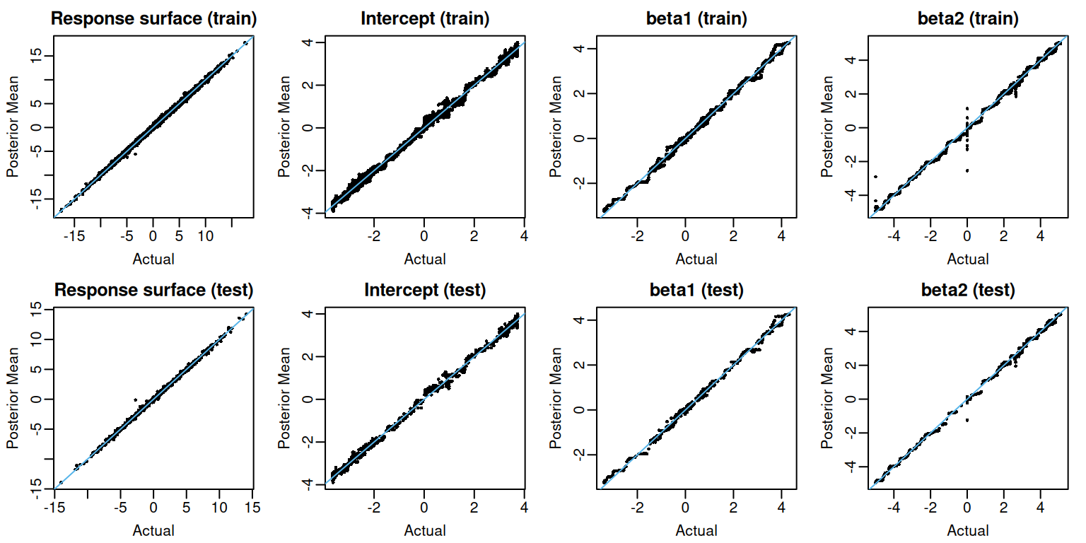

Figure 1: Actual (horizontal) vs Estimated (vertical) evaluations of $\mathbb{E}[Y \vert \boldsymbol{\mathbf{X}},\boldsymbol{\mathbf{Z}}]$ and the individual coefficient functions $\beta_{0}(\boldsymbol{\mathbf{X}}), \beta_{1}(\boldsymbol{\mathbf{X}}),$ and $\beta_{2}(\boldsymbol{\mathbf{X}}).$

Pointwise Uncertainty

When the optional argument save_samples is set to TRUE (the default setting), flexBART::flexBART returns the posterior samples of the response surface and individual covariate function evaluations at each training and testing observation. The output attribute yhat.train (resp. yhat.test) is a matrix whose rows index MCMC draws and whose columns index training (resp. testing) observations. We can form posterior credible intervals for evaluations of the response surface $\mathbb{E}[Y \vert \boldsymbol{\mathbf{X}}, \boldsymbol{\mathbf{Z}}]$ at each training (resp. testing) observation by computing quantiles in each column of yhat.train (resp. yhat.test).

mu_train_l95 <- 
  apply(fit$yhat.train, MARGIN = 2, FUN = quantile, probs = 0.025)
mu_train_u95 <- 
  apply(fit$yhat.train, MARGIN = 2, FUN = quantile, probs = 0.975)

mu_test_l95 <- 
  apply(fit$yhat.test, MARGIN = 2, FUN = quantile, probs = 0.025)
mu_test_u95 <- 
  apply(fit$yhat.test, MARGIN = 2, FUN = quantile, probs = 0.975)

For these data, the coverage is quite high

cat("Training coverage: ", round(mean(mu_train >= mu_train_l95 & mu_train <= mu_train_u95), digits = 3), "\n")
#> Training coverage:  0.974
cat("Testing coverage: ", round(mean(mu_test >= mu_test_l95 & mu_test <= mu_test_u95), digits = 3), "\n")
#> Testing coverage:  0.971

The output attribute beta.train (resp. beta.test) is a three-dimensional array whose dimensions respectively index MCMC draws, training (resp. testing) observations, and ensembles (i.e., covariate functions). To form credible intervals for each $\beta_{j}(\boldsymbol{\mathbf{x}}_{i})$ , we must compute column-wise quantiles in the corresponding slice of beta.train or beta.test.

beta_train_l95 <-
  apply(fit$beta.train, MARGIN = c(2,3), FUN = quantile, probs = 0.025)
beta_train_u95 <-
  apply(fit$beta.train, MARGIN = c(2,3), FUN = quantile, probs = 0.975)
beta_test_l95 <-
  apply(fit$beta.test, MARGIN = c(2,3), FUN = quantile, probs = 0.025)
beta_test_u95 <-
  apply(fit$beta.test, MARGIN = c(2,3), FUN = quantile, probs = 0.975)

The coverage of these intervals is also quite good.

coverage <- 
  matrix(nrow = 2, ncol = 3,
         dimnames = list(c("train", "test"),
                         c("beta0", "beta1", "beta2")))
coverage["train", "beta0"] <-
  mean(beta0_train >= beta_train_l95[,1] & beta0_train <= beta_train_u95[,1])
coverage["train", "beta1"] <-
  mean(beta1_train >= beta_train_l95[,2] & beta1_train <= beta_train_u95[,2])
coverage["train", "beta2"] <-
  mean(beta2_train >= beta_train_l95[,3] & beta2_train <= beta_train_u95[,3])

coverage["test", "beta0"] <-
  mean(beta0_test >= beta_test_l95[,1] & beta0_test <= beta_test_u95[,1])
coverage["test", "beta1"] <-
  mean(beta1_test >= beta_test_l95[,2] & beta1_test <= beta_test_u95[,2])
coverage["test", "beta2"] <-
  mean(beta2_test >= beta_test_l95[,3] & beta2_test <= beta_test_u95[,3])

print(round(coverage, digits = 3))
#>       beta0 beta1 beta2
#> train 0.974 0.963 0.979
#> test  0.976 0.967 0.973

Variable Selection

As we did in the Getting Started article, we can compute the marginal posterior probability inclusion probability that each $X_{j}$ is used in at least one splitting rule in the ensemble for each $\beta_{r}(\boldsymbol{\mathbf{X}}).$ We can then select those $X_{j}$ ’s for which this probability exceeds 50%.

The varcounts element of flexBART()’s output is an array holding the posterior samples of the counts of rules based on each $X_{j}.$ The dimensions of this array, respectively, index MCMC draws, elements of $\boldsymbol{\mathbf{X}}$ , and ensembles/coefficient functions (i.e., $\beta_{0}, \ldots, \beta_{R-1}$ ).

dim(fit$varcounts)
#> [1] 4000   20    3

The selected variables are

pip <- 
  apply(fit$varcounts >= 1, MARGIN = c(2,3), FUN = mean)
which(pip >= 0.5, arr.ind = TRUE)
#>     row col
#> X1    1   1
#> X11  11   1
#> X1    1   2
#> X1    1   3

We see that $X_{1}$ and $X_{11}$ are selected for $\beta_{0};$ $X_{1}$ is selected for $\beta_{2};$ and $X_{1}$ is selected for $\beta_{3}.$ So, at least for this run, there is no false positive and no false negative identifications.

Plotting Coefficient Functions

Although $\boldsymbol{\mathbf{X}}$ contains $p = 20$ predictors, these coefficient functions only depend on $X_{1}$ and $X_{11}.$ So, we can visualize these functions pretty easily. To do so, we first define a new data frame containing a fine grid of $X_{1}$ values, two different $X_{11}$ values (which induce different $\beta_{0}(\boldsymbol{\mathbf{X}})$ values), and dummy values for the remaining predictors and covariates.

x1_seq <- seq(from = -1, to = 1, by = 0.01)
n1 <- length(x1_seq)

plot_df <- data.frame(X1 = c(x1_seq, x1_seq))
for(j in 2:p_cont) plot_df[,paste0("X",j)] <- runif(2*n1, -1, 1)
plot_df[,"X11"] <- 
  factor(c(rep(1, times = n1), rep(3, times = n1)), levels = 1:10)
for(j in 2:p_cat){
  plot_df[,paste0("X",p_cont+j)] <- 
    factor(sample(1:10, size = 2*n1, replace = TRUE), levels = 1:10)
}
plot_df[,"Z1"] <- rnorm(n = 2*n1, mean = 0, sd = 1)
plot_df[,"Z2"] <- rnorm(n = 2*n1, mean = 0, sd = 1)

We then evaluate the coefficient functions on this data frame

beta0_plot <- beta0_true(plot_df)
beta1_plot <- beta1_true(plot_df)
beta2_plot <- beta2_true(plot_df)

We can now plot the three true coefficient functions.

Code


ix0 <- 1:n1
ix1 <- (n1+1):(2*n1)
par(mar = c(3,3,2,1), mgp = c(1.8, 0.5, 0), mfrow = c(1,3))

plot(1, type = "n", xlim = c(-1,1), ylim = c(-5,5),
     main = "Intercept", xlab = "X1", ylab = "beta0")
lines(x1_seq, beta0_plot[ix0], lty = 1)
lines(x1_seq, beta0_plot[ix1], lty = 2)

legend("bottomright", 
       legend = "X11 in {1,2,5,6,9}", lty = 1, bty = "n")
legend("topleft", 
       legend = "X11 in {3,4,7,8,10}",
       lty = 2, bty = "n")

plot(1, type = "n", xlim = c(-1,1), ylim = c(-5,5),
     main = "Effect of Z1", xlab = "X1", ylab = "beta1")
lines(x1_seq, beta1_plot[ix0])

ix2_0 <- which(x1_seq < -0.5)
ix2_1 <- which(x1_seq >= -0.5 & x1_seq < 0.2)
ix2_2 <- which(x1_seq >= 0.2)
plot(1, type = "n", xlim = c(-1,1), ylim = c(-5,5),
     main = "Effect of Z2", xlab = "X1", ylab = "beta2")
lines(x1_seq[ix2_0], beta2_plot[ix2_0])
lines(x1_seq[ix2_1], beta2_plot[ix2_1])
lines(x1_seq[ix2_2], beta2_plot[ix2_2])
lines(x = c(-0.5, -0.5), y = c(beta2_plot[50], beta2_plot[51]), lty = 3)
lines(x = c(0.2, 0.2), y = c(beta2_plot[121], beta2_plot[122]), lty = 3)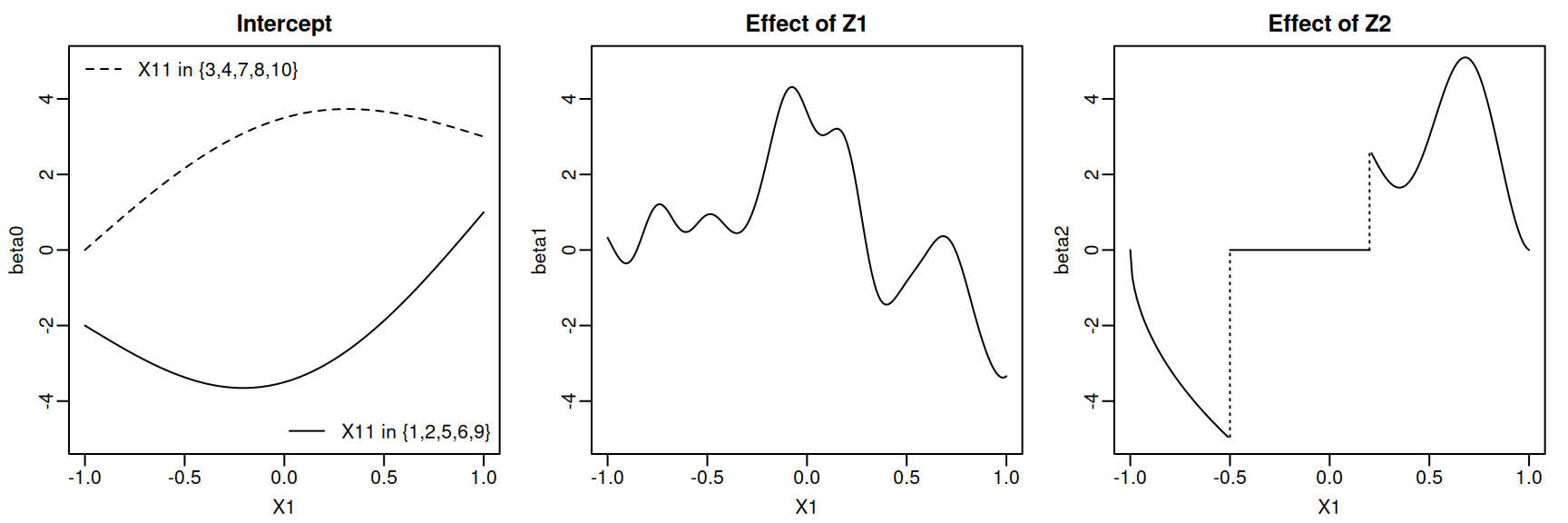

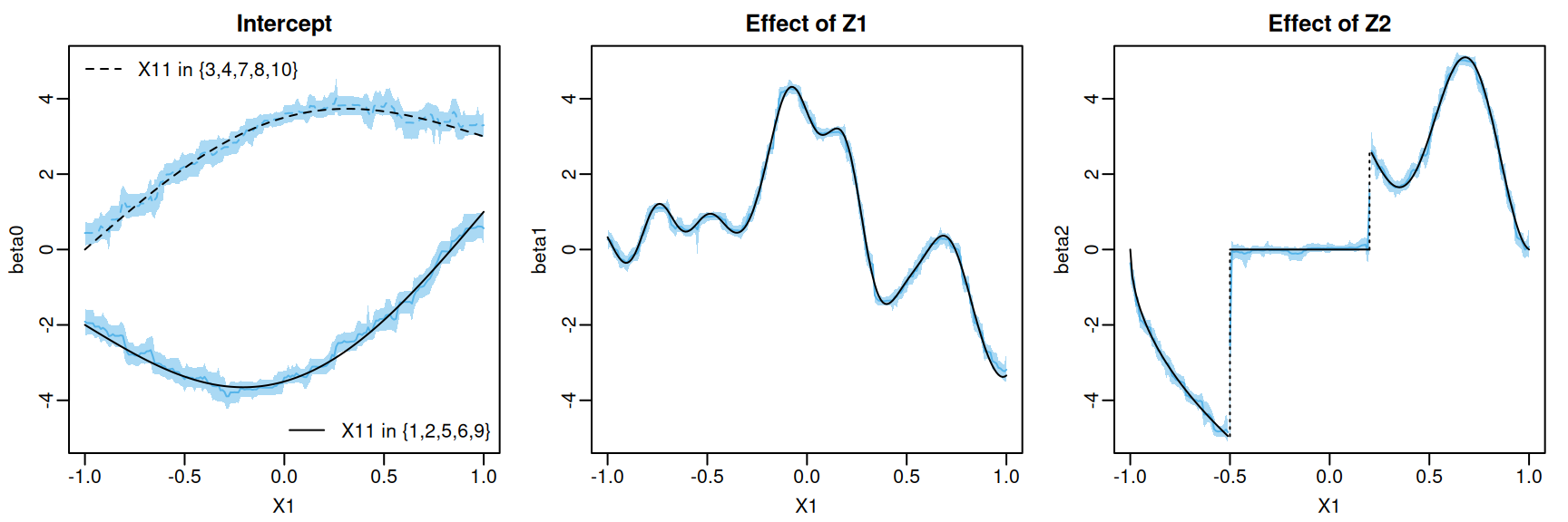
We can also plot the posterior mean and pointwise uncertainty intervals. To do this, we will pass our plot_df data frame to flexBART’s predict method. The output attribute beta is an array containing the MCMC samples of each coefficient function evaluated at every observation in plot_df

plot_fit <- predict(object = fit, newdata = plot_df)
dim(plot_fit$beta)
#> [1] 4000  402    3

We can get the posterior mean and 95% pointwise credible intervals for each evaluation.

Code

beta0_summary <-
  data.frame(
    MEAN = apply(plot_fit$beta[,,1], MAR = 2, FUN = mean),
    L95 = apply(plot_fit$beta[,,1], MAR = 2, FUN = quantile, probs = 0.025),
    U95 = apply(plot_fit$beta[,,1], MAR = 2, FUN = quantile, probs = 0.975))

beta1_summary <-
  data.frame(
    MEAN = apply(plot_fit$beta[,,2], MAR = 2, FUN = mean),
    L95 = apply(plot_fit$beta[,,2], MAR = 2, FUN = quantile, probs = 0.025),
    U95 = apply(plot_fit$beta[,,2], MAR = 2, FUN = quantile, probs = 0.975))

beta2_summary <-
  data.frame(
    MEAN = apply(plot_fit$beta[,,3], MAR = 2, FUN = mean),
    L95 = apply(plot_fit$beta[,,3], MAR = 2, FUN = quantile, probs = 0.025),
    U95 = apply(plot_fit$beta[,,3], MAR = 2, FUN = quantile, probs = 0.975))

We can visualize the posterior mean and pointwise credible intervals of each coefficient function.

Code


par(mar = c(3,3,2,1), mgp = c(1.8, 0.5, 0), mfrow = c(1,3))
plot(1, type = "n", xlim = c(-1,1), ylim = c(-5,5),
     main = "Intercept", xlab = "X1", ylab = "beta0")

polygon(x = c(x1_seq, rev(x1_seq)),
        y = c(beta0_summary$L95[ix0], rev(beta0_summary$U95[ix0])),
        col = adjustcolor(oi_colors[3], alpha.f = 0.5),
        border = NA)

polygon(x = c(x1_seq, rev(x1_seq)),
        y = c(beta0_summary$L95[ix1], rev(beta0_summary$U95[ix1])),
        col = adjustcolor(oi_colors[3], alpha.f = 0.5),
        border = NA)

lines(x1_seq, beta0_summary$MEAN[ix0], col = oi_colors[3])
lines(x1_seq, beta0_summary$MEAN[ix1], col = oi_colors[3], lty = 2)

lines(x1_seq, beta0_plot[ix0], lty = 1)
lines(x1_seq, beta0_plot[ix1], lty = 2)

legend("bottomright", 
       legend = "X11 in {1,2,5,6,9}", lty = 1, bty = "n")
legend("topleft", 
       legend = "X11 in {3,4,7,8,10}",
       lty = 2, bty = "n")

plot(1, type = "n", xlim = c(-1,1), ylim = c(-5,5),
     main = "Effect of Z1", xlab = "X1", ylab = "beta1")

polygon(x = c(x1_seq, rev(x1_seq)),
        y = c(beta1_summary$L95[ix0], rev(beta1_summary$U95[ix0])),
        col = adjustcolor(oi_colors[3], alpha.f = 0.5),
        border = NA)

lines(x1_seq, beta1_summary$MEAN[ix0], col = oi_colors[3])
lines(x1_seq, beta1_plot[ix0])

plot(1, type = "n", xlim = c(-1,1), ylim = c(-5,5),
     main = "Effect of Z2", xlab = "X1", ylab = "beta2")


polygon(x = c(x1_seq[ix2_0], rev(x1_seq[ix2_0])),
        y = c(beta2_summary$L95[ix2_0], rev(beta2_summary$U95[ix2_0])),
        col = adjustcolor(oi_colors[3], alpha.f = 0.5),
        border = NA)

lines(x1_seq[ix2_0], beta2_summary$MEAN[ix2_0], col = oi_colors[3])
lines(x1_seq[ix2_0], beta2_plot[ix2_0])


polygon(x = c(x1_seq[ix2_1], rev(x1_seq[ix2_1])),
        y = c(beta2_summary$L95[ix2_1], rev(beta2_summary$U95[ix2_1])),
        col = adjustcolor(oi_colors[3], alpha.f = 0.5),
        border = NA)

lines(x1_seq[ix2_1], beta2_summary$MEAN[ix2_1], col = oi_colors[3])
lines(x1_seq[ix2_1], beta2_plot[ix2_1])

polygon(x = c(x1_seq[ix2_2], rev(x1_seq[ix2_2])),
        y = c(beta2_summary$L95[ix2_2], rev(beta2_summary$U95[ix2_2])),
        col = adjustcolor(oi_colors[3], alpha.f = 0.5),
        border = NA)

lines(x1_seq[ix2_2], beta2_summary$MEAN[ix2_2], col = oi_colors[3])
lines(x1_seq[ix2_2], beta2_plot[ix2_2])


lines(x = c(-0.5, -0.5), y = c(beta2_plot[50], beta2_plot[51]), lty = 3)
lines(x = c(0.2, 0.2), y = c(beta2_plot[121], beta2_plot[122]), lty = 3)

Figure 3: True coefficient functions (black) and the posterior mean and 95% pointwise credible intervals (blue).