fan_walk <- function(init_state, n_iter, P){
  states <- colnames(P)
  states_visited <- rep(NA, times = n_iter)
  states_visited[1] <- init_state
  for(r in 2:n_iter){
    states_visited[r] <-
      sample(states, size = 1,
             prob = P[states_visited[r-1],])
  }
  props <- table(states_visited)[states]/n_iter
  return(props)
}STAT 479 Lecture 15
Markov Chains II
Overview
- Lecture 14: Markov chain model of baseball
- Estimated transition probabilities b/w out-baserunner states
- Single absorbing state
3.000: once reached, chain never leaves - Simulation: inning length & expected runs
- Theory: # at-bats until end of inning
- Today: using Markov chains to rank teams
- Simulate a random walk (Markov chain) b/w teams
- \(p_{s,s'}\) tracks how much better \(s'\) is than \(s\)
- Essentially, a variant of PageRank, which used to power Google Search
Modeling a Bandwagon Fan
- Bandwagon fan: supports an actively successful/trendy team, no past loyalty,
- Imagine a bandwagon fan randomly switching support b/w \(S\) teams
- Each day, fan switches their support to a different team
- \(p_{s,s'}\): prob. of switching from \(s\) to \(s'\)
- Long-term behavior: how often does fan support any one team?
4 Team Example: Setup
- Markov chain model of fan’s support:
- Each day, stay with same team or pick different one
- Transitions depend only on current team (not past)
4 Team Example: Simulation Function
- Function to compute long-run frequencies for each team
- Arguments: initial state, number of iterations, transition matrix
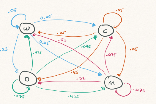
4 Team Example: Simulation
teams <- c("W", "O", "C", "M")
P <- matrix(c(0.05, 0.85, 0.05, 0.05,
              0.425, 0.075, 0.075, 0.425,
              0.05, 0.85, 0.05, 0.05,
              0.53, 0.32, 0.075, 0.075),
            byrow = TRUE, nrow = 4, ncol = 4,
            dimnames = list(teams, teams))

set.seed(479)
round(fan_walk(init_state = "W", n_iter = 1e6, P = P), digits = 3)
states_visited
W O C M
0.307 0.416 0.066 0.211 Additional Markov Chain Theory
Setup
- \(\{X_{t}\}\) Markov chain over \(\mathcal{S} = \{1, 2, \ldots, S\}\)
- Transition matrix \(\boldsymbol{\mathbf{P}}\)
- \(p_{s,s'} = \mathbb{P}(X_{t+1} = s' \vert X_{t} = s)\)
- \(n\)-step transition matrix: \(\boldsymbol{\mathbf{P}}^{n}\)
- \((\boldsymbol{\mathbf{P}}^{n})_{s,s'} = \mathbb{P}(X_{t+n} = s' \vert X_{t} = s)\)
- Sums over all possible \(n\)-step paths from \(s\) to \(s'\)
\(n\)-step Distribution I
- Suppose we randomly initialize according to \(\boldsymbol{\pi}_{0} = (\pi_{0,1}, \ldots, \pi_{0,S})^{\top}\)
- I.e. for all \(s\), \(\pi_{0,s} = \mathbb{P}(X_{0} = s)\)
- What is \(\mathbb{P}(X_{1} = s')\) for all \(s'\)?
\[ \begin{align} \mathbb{P}(X_{1} = s') &= \sum_{s}{\mathbb{P}(X_{1} = s', X_{0} = s)} \\ &= \sum_{s}{\mathbb{P}(X_{0} = s) \times \mathbb{P}(X_{1} = s' \vert X_{0} = s)} \\ &= \sum_{s}{\pi_{0,s} \times p_{s,s'}} \end{align} \]
\(n\)-step Distribution II
- \(\boldsymbol{\pi}_{1} = (\pi_{1,1}, \ldots, \pi_{1,S})^{\top}\) where \(\pi_{1,s} = \mathbb{P}(X_{1} = s)\)
- \(\boldsymbol{\pi}_{1}^{\top} = \boldsymbol{\pi}_{0}^{\top}\boldsymbol{\mathbf{P}}\)
Using almost identical calculations: \(\boldsymbol{\pi}_{n}^{\top} = \boldsymbol{\pi}_{n-1}^{\top}\boldsymbol{\mathbf{P}} = \boldsymbol{\pi}_{0}^{\top}\boldsymbol{\mathbf{P}}^{n}.\)
Limiting distribution \(\lim_{n \rightarrow \infty} \boldsymbol{\pi}_{n}\)
- Long-term prop. of time spend in each state
- Does not necessarily exist
Invariant Distribution
- If \(\boldsymbol{\pi}^{\top} = \boldsymbol{\pi}^{\top}\boldsymbol{\mathbf{P}}\), we say \(\boldsymbol{\pi}\) is invariant
- Say \(\boldsymbol{\pi}\) is invariant: if \(X_{t} \sim \boldsymbol{\pi}\) then for all \(n\) \(X_{t+n} \sim \boldsymbol{\pi}\)
- If limiting distribution exists, it is invariant!
Existence of Limiting Distribution
- \(\{X_{t}\}\) has a unique, limiting distribution if it is
- Irreducible: possible to move b/w any \(s\) & \(s'\) in finitely many steps
- Aperiodic: can return to \(s\) at any time and not on fixed schedule
- Positive recurrent: chain returns to \(s\) in finitely many steps w.p. 1
- Compute invariant distribution by finding leading left eigenvector
4-Team Example: Invariant Distribution
get_invariant <- function(P, tol = 1e-12){
  states <- colnames(P)
  if(!all( abs(rowSums(P) - 1) < tol) ){
    stop("Rows sums of P are not all 1. P may not be a valid transition matrix") #<2
  }

  decomp <- eigen(t(P))
  pi_raw <- decomp$vectors[,1]

  if(!all(Re(pi_raw) < tol)){
    stop("Leading eigenvalue of P appears to be complex and not real-valued")
  }
  pi <- Re(pi_raw)
  pi <- pi/sum(pi)
  names(pi) <- states

  return(pi)
}
pi: 0.307308 0.415808 0.065675 0.211208 pi %*% P: 0.307308 0.415808 0.065675 0.211208 Difference: -5.551115e-17 -2.220446e-16 1.387779e-17 2.220446e-16 Recipe: Markov chain-based rankings:
- Construct aperiodic, irreducible, positive recurrent Markov chain over teams
- Compute invariant distribution
- No one way to construct the chain
- Intuition: \(p_{s,s'}\) should capture how much better \(s'\) is than \(s\)
Win Matrix
- Let \(v_{s,s'}\) be # times team \(s\)’ beats team \(s\)
- Arrange \(v_{s,s'}\) values into \(S \times S\) matrix \(\boldsymbol{\mathbf{V}}\)
- \(\boldsymbol{\mathbf{W}}\): normalize rows of \(\boldsymbol{\mathbf{V}}\) to have sum 1
- Tempting to use \(\boldsymbol{\mathbf{W}}\) as transition matrix
- Problem: resulting Markov chain may not have invariant distribution
Dampening
- Fix some \(0 < \beta < 1\) \[ \boldsymbol{\mathbf{P}} = \beta \times \boldsymbol{\mathbf{W}} + \frac{(1 - \beta)}{S} \times \mathbf{\boldsymbol{1}}_{S}^{\top}\mathbf{\boldsymbol{1}}_{S} \]
- Multiply all elements of \(\boldsymbol{\mathbf{W}}\) by \(\beta\)
- Add \((1-\beta)/S\) to all entries of re-scaled \(\boldsymbol{\mathbf{W}}\)
- Usually ensures positive recurrence, aperiodicity, and irreducibility
NCAA Hockey Ranking: Setup
load("wd1hockey_regseason_2024_2025.RData")
teams <- sort(unique(c(no_ties$Home, no_ties$Opponent)))
S <- length(teams)

results <-
  no_ties |>
  dplyr::rename(
    home.team = Home, home.score = HomeScore,home.winner = Home_Winner,
    away.team = Opponent, away.score = OppScore, away.winner = Opp_Winner) |>
  dplyr::select(home.team, away.team, home.winner, away.winner, home.score, away.score)
NCAA Hockey Rankings: \(\boldsymbol{\mathbf{V}}\)
           Wisconsin Ohio State Minnesota Cornell
Wisconsin          0          2         0       0
Ohio State         2          0         2       0
Minnesota          5          3         0       0
Cornell            0          1         0       0
V <- matrix(0, nrow = S, ncol = S, dimnames = list(teams, teams))
for(i in 1:nrow(results)){
home <- results$home.team[i]
away <- results$away.team[i]
if(results$home.winner[i] == 1){
V[away,home] <- V[away,home] + 1
} else if(results$away.winner[i] == 1){
V[home,away] <- V[home,away] + 1
} else{
cat("Problem with game", i, ": neither team won")
}
}Dampening Function
NCAA Hockey Rankings
- WIS only lost to OSU: massive transition prob. from
WIStoOSU
P <- get_dampened_transition(V, beta = 0.85)
P[c("Wisconsin", "Ohio State", "Cornell", "Minnesota"), c("Wisconsin", "Ohio State", "Cornell", "Minnesota")]
Wisconsin Ohio State Cornell Minnesota
Wisconsin 0.003409091 0.853409091 0.003409091 0.003409091
Ohio State 0.215909091 0.003409091 0.003409091 0.215909091
Cornell 0.003409091 0.173409091 0.003409091 0.003409091
Minnesota 0.357575758 0.215909091 0.003409091 0.003409091Alternative: Score-based transitions
- \(v_{s,s'}\): number of goals scored by \(s\)’ when playing \(s\)
- Sum of \(s\)-th row of \(\boldsymbol{\mathbf{V}}\): goals conceded by team \(s\)
- Sum of \(s\)-th column of \(\boldsymbol{\mathbf{V}}\): goals scored by team \(s\)
- Intuition: encourage transition if \(s'\) scores a lot against \(s\)
Scored-Based Rankings
V_score <- matrix(0, nrow = S, ncol = S, dimnames = list(teams, teams))
for(i in 1:nrow(results)){
  home <- results$home.team[i]
  away <- results$away.team[i]

  V_score[away, home] <- V_score[away,home] + results$home.score[i]
  V_score[home,away] <- V_score[home,away] + results$away.score[i]
}
V[c("Wisconsin", "Ohio State", "Cornell", "Minnesota"), c("Wisconsin", "Ohio State", "Cornell", "Minnesota")]
Wisconsin Ohio State Cornell Minnesota
Wisconsin 0 2 0 0
Ohio State 2 0 0 2
Cornell 0 1 0 0
Minnesota 5 3 0 0- Manually adjusted \(\beta = 0.5\) to ensure numerical stability
P_score <- get_dampened_transition(V_score, beta = 0.8)
pi_score <- get_invariant(P_score)
round(sort(pi_score, decreasing = TRUE), digits = 3)[1:10]
Wisconsin Minnesota Ohio State Colgate
0.053 0.048 0.045 0.039
Cornell Minnesota Duluth Minnesota State Clarkson
0.034 0.033 0.030 0.029
St. Lawrence Princeton
0.029 0.028 Remarks
- Markov chain-based rankings very popular among operations researchers
- Early papers on ranking college basketball & football
- Differ in construction of \(\boldsymbol{\mathbf{V}}\)
- Badger Bracketology : run by Prof. Laura Albert (ISy&E)
- Markov chain model to obtain team rankings (i.e., invariant \(\pi_{s}\)’s)
- Simulate games according to \(\mathbb{P}(s' \textrm{ beats } s) = \frac{\pi_{s}}{\pi_{s} + \pi_{s'}}.\)
- Markov chain based rankings are very sensitive to choices (\(\boldsymbol{\mathbf{V}}\), \(\beta\), etc.)
- Personally, I prefer model-based rankings (e.g., Bradley-Terry)
- Directly quantify uncertainty about observables
- Simulation in probabilistically coherent fashion