# A tibble: 8 × 6
  at_bat_number  Outs BaseRunner end_events      end_Outs end_BaseRunner
          <int> <int> <chr>      <chr>              <dbl> <chr>
1            59     0 000        walk                   0 100
2            60     0 100        single                 0 110
3            61     0 110        walk                   0 111
4            62     0 111        sac_fly                1 110
5            63     1 110        fielders_choice        1 110
6            64     1 110        single                 1 110
7            65     1 110        single                 1 110
8 66 1 110 double_play 3 <NA> STAT 479 Lecture 14
Markov Chains
State Transitions in Baseball
- 8th inning of Dodgers-Padres game on March 20, 2024
- Game state transitions:
0.000to0.100to0.110to0.111to1.110- Eventually transitions from
1.110to3.000(end of inning)
Motivation & Objectives
- How unusual was this sequence of state transitions?
- If we replayed inning over and over again, how many at-bats?
- Dist. of runs scored?
- Given the game is in
1.000, how likely is it to reach2.111?
- Today: a probabilistic model for state transitions
Data Preparation
- For every at bat, record starting state and ending state
- Also useful to create table of 25 unique game states (see lecture notes)
Markov Chains Fundamentals
Setting
- State space: \(\mathcal{S} = \{1, 2, \ldots, S\}\)
- \(\{X_{t}\}\): infinite sequence of \(\mathcal{S}\)-valued random variables
- Interested in several probabilities & random quantities
- \(\mathbb{P}(X_{1} = s_{1}, X_{2} = s_{2}, X_{3} = s_{3}, X_{4} = s_{4}\)): e.g., likelihood of seeing
0.000to1.000to2.000to3.000 - First \(n\) such that \(X_{n} \in A\): e.g., # at-bats needed to get at least one out
- Amount of time to reach state \(s\) starting from state \(s'\)
- \(\mathbb{P}(X_{1} = s_{1}, X_{2} = s_{2}, X_{3} = s_{3}, X_{4} = s_{4}\)): e.g., likelihood of seeing
Specifying Joint Distributions
- To answer these questions, must define a joint probability distribution:
- For every infinite sequence of states \(s_{1}, s_{2}, \ldots\) must specify \[ \mathbb{P}(X_{1} = s_{1}, X_{2} = s_{2}, X_{3} = s_{3}, \ldots) \]
- Can compute prob. of events of interest by
- Enumerating all infinite sequences for which event occurs
- Sum the probabilities of those sequences
Joints from Conditionals
Specify joint dist. \(\{X_{t}\}\) by specifying sequence of conditional probabilities \[ \mathbb{P}(X_{t+1} = s \vert X_{t} = s_{t}, X_{t-1} = s_{t-1}, X_{t-2} = s_{t-2}, \ldots, X_{1} = s_{1}) \]
Specifying how to generate next value based on all previous values
- To characterize \(X_{t+1}\), must specify a total of \(S \times S^{t}\) different probabilities
- \(S\) possible states for \(X_{t+1}\)
- \(S^{t}\) possible sequences \(s_{1}, \ldots, s_{t}\)
Markov Property
- \(\{X_{t}\}\) satisfies the Markov property if:
- For all \(A \subset \mathcal{A}\)
- For all \(t\) and sequences \(s_{1}, \ldots s_{t}\) \[ \mathbb{P}(X_{t+1} \in A \vert X_{t} = s_{t}, \ldots, X_{1} = s_{1}) = \mathbb{P}(X_{t+1} \in A \vert X_{t} = s_{t}) \]
- What comes next depends only on current state & not past states
Markov Chains
If \(\{X_{t}\}\) satisfies Markov property, we say it is a Markov chain
Markov chains on state space \(\mathcal{S} = \{1, 2, \ldots, S\}\) are determined by transition probability matrix \[ \boldsymbol{\mathbf{P}} = \begin{pmatrix} p_{1,1} & \cdots & p_{1,S} \\ \vdots & ~ & \vdots \\ p_{S,1} & \cdots & p_{S,S} \end{pmatrix} \]
\(p_{s, s'} = \mathbb{P}(X_{t+1} = s' \vert X_{t} = s)\): prob. of moving from \(s\) to \(s'\)
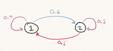
2-State Example
- If chain is
- At
1: move to2w.p. 60% and remain at1w.p. 40% - At
2: move to1w.p. 50% and remain at2w.p. 50%
- At
2-State Example: Simulation
set.seed(479)
states <- c(1,2)
P<- matrix(c(0.6, 0.4, 0.5, 0.5), nrow = 2, ncol = 2, byrow = TRUE)
n_steps <- 10
init_state <- 2
states_visited <- rep(NA, times = n_steps)
states_visited[1] <- init_state
for(t in 2:n_steps){
prev_state <- states_visited[t-1]
probs <- P[prev_state,]
next_state <- sample(states, size = 1, prob = probs)
states_visited[t] <- next_state
}
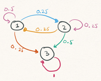
states_visited [1] 2 1 1 1 2 2 2 1 1 23-State Example
- When the chain reaches
3, it remains there.
3-State Example: Simulation
- Simulate the Markov chain 10 times for 10 iterations each
- Each simulation begins in state
1 - All quickly reach state
3(absorbing)
Simulation  1 : 1 3 3 3 3 3 3 3 3 3
Simulation  2 : 1 2 3 3 3 3 3 3 3 3
Simulation  3 : 1 2 2 3 3 3 3 3 3 3
Simulation  4 : 1 2 3 3 3 3 3 3 3 3
Simulation  5 : 1 2 2 1 1 2 3 3 3 3
Simulation  6 : 1 2 3 3 3 3 3 3 3 3
Simulation  7 : 1 2 3 3 3 3 3 3 3 3
Simulation  8 : 1 3 3 3 3 3 3 3 3 3
Simulation  9 : 1 2 1 1 1 1 2 3 3 3
Simulation  10 : 1 1 3 3 3 3 3 3 3 3
3-State Example: Absorbtion Time
- Starting from
1, how long until chain reaches state3? - \(T_{1}^{A} = \min\left\{t \geq 1: X_{t} = 3\right\}\)
- See notes for code
- Simulated 10,000 Markov chains
absorption_time
   2    3    4    5    6    7    8    9   10   11   12   13   14   15   16
2511 3209 1701  995  586  395  226  159   83   52   32   20   12    8    6
A Markov Chain Model for Baseball
Estimating Transition Probabilities
- Focus only on at-bats in the first 8 innings
- \(n_{s,s'}\): number of at-bats starting in state \(s\) and ending in \(s'\)
- \(n_{s}\): number of at-bats starting in state \(s\)
- Estimate \(p_{s,s'}\) with \(n_{s,s'}/n_{s}\)
Baseball Transitions: Visualization
![]()
Half-Inning Simulation
- Start at
0.000and terminate once chain reaches3.000
max_iterations <- 30
states_visited <- rep(NA, times = max_iterations)

iteration_counter <- 1
states_visited[1] <- "0.000"
current_state <- "0.000"
set.seed(479)
while(current_state != "3.000" & iteration_counter < max_iterations){

  current_state <-
    sample(unik_states$GameState, size = 1,
           prob = transition_matrix[current_state,])
  iteration_counter <- iteration_counter + 1
  states_visited[iteration_counter] <- current_state
}
states_visited[1:(iteration_counter)]
[1] "0.000" "0.010" "1.010" "2.010" "2.000" "3.000"Inning-Length Simulation I
- See lecture notes for full code
- Simulated 50,000 half-innings, keeping track of all states visited
      [,1]    [,2]    [,3]    [,4]    [,5]    [,6]    [,7]    [,8]
 [1,] "0.000" "1.000" "2.000" "3.000" NA      NA      NA      NA
 [2,] "0.000" "1.000" "2.000" "2.100" "3.000" NA      NA      NA
 [3,] "0.000" "1.000" "1.100" "2.100" "2.011" "3.000" NA      NA
 [4,] "0.000" "1.000" "2.000" "3.000" NA      NA      NA      NA
 [5,] "0.000" "1.000" "1.100" "3.000" NA      NA      NA      NA
 [6,] "0.000" "1.000" "2.000" "3.000" NA      NA      NA      NA
 [7,] "0.000" "1.000" "2.000" "3.000" NA      NA      NA      NA
 [8,] "0.000" "1.000" "2.000" "2.100" "3.000" NA      NA      NA
 [9,] "0.000" "1.000" "1.100" "2.010" "2.100" "2.110" "3.000" NA
[10,] "0.000" "0.010" "1.001" "1.100" "2.100" "3.000" NA      NA
Inning-Length Simulation II
- For each row of
states_visitedfind first instance3.000
inning_length <-
  apply(states_visited,
        MARGIN = 1,
        FUN = function(x){ return(which(x == "3.000") - 1)} )
table(inning_length)
inning_length
3 4 5 6 7 8 9 10 11 12 13 14 15
19138 14368 8685 4222 2014 921 401 131 72 31 11 4 2 - 2 of the 50,000 simulated half-innings had 15 at-bats
 [1] "0.000" "0.100" "0.110" "1.110" "1.000" "1.100" "1.000" "1.100" "1.000"
[10] "1.000" "1.100" "1.110" "1.101" "2.100" "2.000"
Runs Scored
\(O_{t}\) and \(B_{t}\): number of outs and runners at the start of at-bat \(t\)
\(O^{\star}_{t}\) and \(B^{\star}_{t}\): numbers of outs and runners at the end of at-bat \(t\)
Runs Scored during at-bat \(t\): \[ (O_{t} + B_{t} + 1) - (O_{t}^{\star} + B_{t}^{\star}). \]
Re-run simulation & keep running total of runs scored in each at-bat
runs_scored
    0     1     2     3     4     5     6     7     8     9    10    11    12
19138 14368  8685  4222  2014   921   401   131    72    31    11     4     2
Further Markov Chain Theory
\(n\)-step Transitions I
- Suppose \(X_{t} = s\). What is \(\mathbb{P}(X_{t+2} = s' \vert X_{t} = s)\)?
- Starting from
1.000, chances of being at2.100in exactly 2 at-bats?
- Starting from
- Must sum over all all intermediate states between \(s\) and \(s'\): \[ \begin{align} \mathbb{P}(X_{t+2} = s' \vert X_{t} = s) &= \sum_{k = 1}^{S}{\mathbb{P}(X_{t+2} = s', X_{t+1} = k \vert X_{t} = s)} \\ &= \sum_{k = 1}^{S}{\mathbb{P}(X_{t+2} = s' \vert X_{t+1} = k, X_{t} = s)\mathbb{P}(X_{t+1} = k \vert X_{t} = s)} \end{align} \]
\(n\)-step Transitions II
- By Markov Property \[ \mathbb{P}(X_{t+2} = s' \vert X_{t+1} = k, X_{t} = s) = \mathbb{P}(X_{t+2} = s' \vert X_{t+1} = k) = p_{k,s'} \]
- Conclude that \[ \mathbb{P}(X_{t+2} = s' \vert X_{t} = s) = \sum_{k = 1}^{S}{p_{s,k} p_{k,s'}} \]
- This is just matrix multiplication! \(n\)-step transition probability matrix
\[ \boldsymbol{\mathbf{P}}^{n} = \boldsymbol{\mathbf{P}} ~ \overbrace{\times \cdots \times}^{n \textrm{ times}} ~ \boldsymbol{\mathbf{P}} \]
Example
- Starting from
1.000:- 51% chance inning ends after 2 at-bats
- 27% chance inning is at
2.100after 2 at-bats
Fundamental Matrix
- Suppose chain has \(A\) absorbing states & \(T\) non-absorbing states
- Partition transition matrix as \[
\boldsymbol{\mathbf{P}} = \begin{pmatrix} Q & R \\ 0 & I_{A} \end{pmatrix},
\]
- \(Q\): transitions between non-absorbing states
- \(R\): transitions from non-absorbing to absorbing
- Fundamental Matrix: \(N = (I_{T} - Q)^{-1}\)
Example
- \(n_{s,s'}\): expected number of visits to \(s'\) starting from \(s\) before absorption
- Starting from
0.000, chain visits0.1000.25 times and0.0100.06 times - Starting from
1.000chain returns about
- Starting from
transient_states <- unik_states |> dplyr::filter(GameState != "3.000") |> dplyr::pull(GameState)
Q <- transition_matrix[transient_states, transient_states]
R <- matrix(transition_matrix[transient_states, "3.000"], ncol = 1)
N <- solve(diag(24) - Q)
round(N[1:5, 1:5], digits = 2)
0.000 0.100 0.010 0.001 0.110
0.000 1.05 0.25 0.06 0.01 0.06
0.100 0.05 1.02 0.03 0.01 0.22
0.010 0.04 0.07 1.06 0.01 0.13
0.001 0.06 0.20 0.06 1.01 0.06
0.110 0.05 0.02 0.02 0.01 1.06Row Sums of \(N\)
- \(n_{s,s'}\) number of expected visits to \(s'\) by a chain started at \(s\)
- \(\sum_{s'}{n_{s,s'}}\): expected number of states visited before absorption
- Starting from
1.000, expect about 2.8 more at-bats before end of half-inning
Reminders
- Project 2: simulation of a game, season, tournament, draft, etc.
- Simulation powered by a probabilistic model
- Could build a Bradley-Terry, Markov chain, or Plackett-Luce model
- By October 22 (Wednesday): email me w/ your team’s plans!
- Due November 7
- Project 3: Big Data Bowl or curling data
- Big Data Bowl: how players move when ball in air
- Curling: strategies for power play and/or shot selection
- Can work w/ other students (form groups on Canvas)
- By October 22 (Wednesday): email me w/ group & choice of topic
Guest Speaker
- Thursday October 30: David Radke (Chicago Blackhawks)
- 2:30pm - 3:30pm: Research Talk
- “Multiagent Challenges in Team Sports Analytics”
- Aimed at graduate students & faculty but all welcome!
- 3:30pm - 4:30pm: Career Talk
- “Professional Hockey Analytics at the Chicago Blackhawks”
- How does Hockey Strateegy & Analytics groups operate?
- Both talks in Morgridge Hall 7560