STAT 479 Lecture 9

Multilevel Models

Motivation

Comparing Football Plays

Which of these two touchdown plays is more impressive?
- 86-yard touchdown pass from Justin Herbert to Ladd McConckey (video link)
- 64-yard touchdown pass from Cooper Rush to KaVontae Turpin (video link)

Plays share many similarities but important differences
- Context: down & distance, time left, score
- Time of pass: number of pass rushers, pocket integrity
- Receiver’s actions after the catch

Today: expected points facilitated nuanced comparison
Multilevel models to determine which passers generate most EP per attempt

Use the nflfastR package

pbp2024 <- nflfastR::load_pbp(season = 2024)

# A tibble: 10 × 5
   game_id          week season_type home_team away_team
   <chr>           <int> <chr>       <chr>     <chr>    
 1 2024_08_NYG_PIT     8 REG         PIT       NYG      
 2 2024_08_MIN_LA      8 REG         LA        MIN      
 3 2024_15_NE_ARI     15 REG         ARI       NE       
 4 2024_10_CIN_BAL    10 REG         BAL       CIN      
 5 2024_01_GB_PHI      1 REG         PHI       GB       
 6 2024_08_KC_LV       8 REG         LV        KC       
 7 2024_03_SF_LA       3 REG         LA        SF       
 8 2024_18_NYG_PHI    18 REG         PHI       NYG      
 9 2024_11_BAL_PIT    11 REG         PIT       BAL      
10 2024_09_NO_CAR      9 REG         CAR       NO

# A tibble: 10 × 7
   time  posteam_score defteam_score side_of_field yardline_100  down ydstogo
   <chr>         <dbl>         <dbl> <chr>                <dbl> <dbl>   <dbl>
 1 10:23             0             0 NYG                     13     4      11
 2 02:40            28            20 LA                      53     2      10
 3 12:24             0             0 ARI                     33     3       5
 4 12:58             0             0 CIN                     56     3       9
 5 05:34            13            12 GB                      15    NA       0
 6 02:00            NA            NA <NA>                    NA    NA       0
 7 15:00             7            14 LA                      70     1      10
 8 00:00             7             0 <NA>                    NA    NA       0
 9 13:27             9             7 PIT                     58     2       7
10 04:13            12             7 CAR                     15    NA       0

# A tibble: 10 × 2
   play_type   desc                                                             
   <chr>       <chr>                                                            
 1 field_goal  (10:23) 9-C.Boswell 31 yard field goal is GOOD, Center-46-C.Kunt…
 2 run         (2:40) 17-P.Nacua right end to LA 45 for -2 yards (7-B.Murphy, 4…
 3 no_play     (12:24) (Shotgun) 4-A.Gibson left tackle pushed ob at ARI 18 for…
 4 pass        (12:58) (Shotgun) 9-J.Burrow pass deep middle to 1-J.Chase to BA…
 5 extra_point 4-J.Elliott extra point is GOOD, Center-49-R.Lovato, Holder-10-B…
 6 no_play     Timeout #2 by LV at 02:00.                                       
 7 pass        (15:00) (Shotgun) 9-M.Stafford pass short middle to 88-J.Whittin…
 8 <NA>        END QUARTER 1                                                    
 9 pass        (13:27) (No Huddle) 3-R.Wilson pass short middle to 30-J.Warren …
10 extra_point 19-B.Grupe extra point is GOOD, Center-49-Z.Wood, Holder-43-M.Ha…

Also several indicators: fumble, complete_pass, passing_yards
Check out the full listing

Player ID

nflfastR uses unique 9-digit id for each player (gsis_id)

roster2024 <-
  nflfastR::fast_scraper_roster(seasons = 2024)

roster2024 |>
  dplyr::filter(full_name == "Jordan Love") |>
  dplyr::select(full_name, gsis_id)

# A tibble: 1 × 2
  full_name   gsis_id   
  <chr>       <chr>     
1 Jordan Love 00-0036264

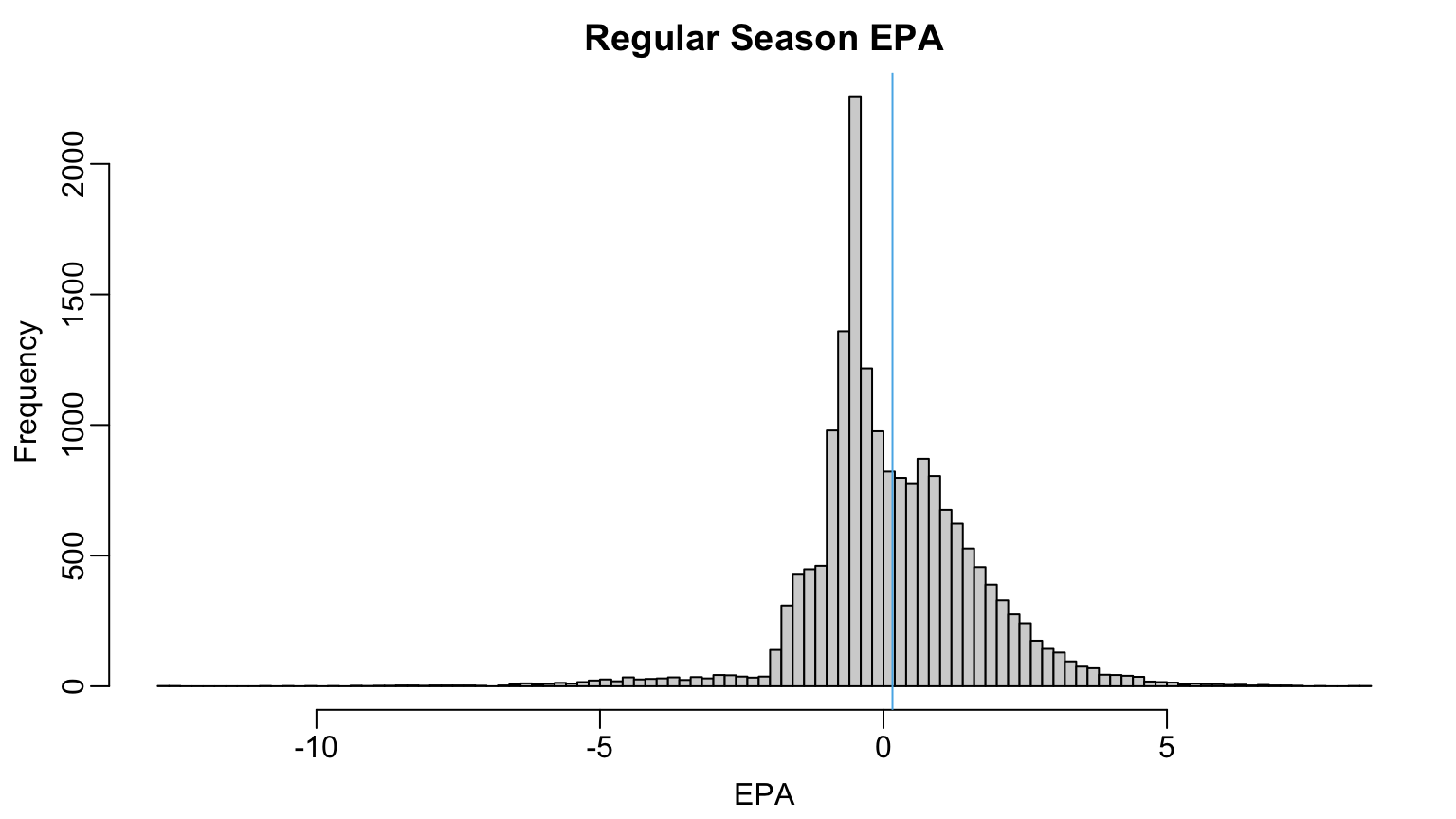
Expected Points

Overivew

Goal: estimate avg. number of points eventually scored by teams from similar situation
EPA: diff. in post- and pre-play EP
- $\textrm{EPA} > 0$: successful for offense
- $\textrm{EPA} < 0$: unsuccessful for offense
nflfastR’s EP model to predict next scoring event in half
- Touchdown (7), field goal (3), safety (2)
- Opposing touchdown (-7), field goal (-3), and safety (-2)
- No score (0)

Expected Points

Vector of next score probabilities given play features $\boldsymbol{\mathbf{z}}$: $\boldsymbol{\pi}(\boldsymbol{\mathbf{z}}) = (\pi_{\textrm{TD}}(\boldsymbol{\mathbf{z}}), \ldots, \pi_{\textrm{oppFG}}(\boldsymbol{\mathbf{z}}))$
Estimated w/ regression tree ensemble using XGBoost

Definition: Expected Points

Given a game state feature vector $\boldsymbol{\mathbf{z}}$ and vector of drive outcome probabilities $\boldsymbol{\pi}(\boldsymbol{\mathbf{z}}),$ the expected points $\textrm{EP}(\boldsymbol{\mathbf{z}})$ is \[ \begin{align} \textrm{EP}(\boldsymbol{\mathbf{z}}) &= 7\times\pi_{\textrm{TD}}(\boldsymbol{\mathbf{z}}) + 3\times\pi_{\textrm{FG}}(\boldsymbol{\mathbf{z}}) + 2\times\pi_{\textrm{SAF}}(\boldsymbol{\mathbf{z}}) \\ ~&~~-2\times\pi_{\textrm{oSAF}}(\boldsymbol{\mathbf{z}}) - 3\times\pi_{\textrm{oFG}}(\boldsymbol{\mathbf{z}}) - 7\times\pi_{\textrm{oTD}}(\boldsymbol{\mathbf{z}}) \end{align} \]

Basic Use: Comparing Plays

ep and epa: starting EP and EP added during play
McConkey TD had highest EPA: 7 - (-1.54) = 8.54
Turpin TD had EPA 7 - 0.77 = 6.23

pbp2024 |>
  dplyr::slice_max(epa) |>
  dplyr::select(ep, epa, desc)

# A tibble: 1 × 3
     ep   epa desc                                                              
  <dbl> <dbl> <chr>                                                             
1 -1.54  8.54 (10:50) (Shotgun) 10-J.Herbert pass deep middle to 15-L.McConkey …

Basic Uses: Comparing Teams

oi_colors <- 
  palette.colors(palette = "Okabe-Ito")
pbp2024 |>
  dplyr::group_by(posteam) |>
  dplyr::summarize(epa = mean(epa, na.rm = TRUE)) |> 
  dplyr::arrange(desc(epa)) |>
  dplyr::slice(c(1:5, (dplyr::n()-4):(dplyr::n())))

# A tibble: 10 × 2
   posteam     epa
   <chr>     <dbl>
 1 BAL      0.143 
 2 BUF      0.141 
 3 DET      0.135 
 4 WAS      0.115 
 5 TB       0.103 
 6 NE      -0.0643
 7 NYG     -0.0829
 8 TEN     -0.0896
 9 LV      -0.107 
10 CLE     -0.151

Predicting EPA on a New Pass

League-Average

EPA on a future pass if you don’t know anything else?
League average mean(pbp2024$epa) seems reasonable

Figure 1: EPA on all regular season passes

Player-Specific Model

Would your prediction change if you knew passer identity?
- If Patrick Mahomes was throwing the pass, expect higher EPA
- If Daniel Jones was throwing the pass, expect lower EPA

$I$: number of unique passers in data set
$Y_{ij}$: EPA on pass $j$ thrown by player $i$
$\alpha_{i}$: avg. EPA/pass for player $i$ (unknown)
Model: $Y_{ij} = \alpha_{i} + \epsilon_{ij}$

Estimating $\alpha_{i}$

Idea 1: group by passer_player_id & compute mean(epa) for each player
Equivalent (and more extensible): fit a linear model w/ least squares

Setup
Estimation
Example
Top-10

Regress epa on categorical passer_player_id
Must convert passer_player_id to a factor()
Useful to manually set a reference player (e.g., Aaron Rodgers)

rodgers_id <- 
  roster2024 |> 
  dplyr::filter(full_name == "Aaron Rodgers") |> 
  dplyr::pull(gsis_id)

pass2024 <-
  pass2024 |>
  dplyr::mutate(
    passer_player_id = factor(passer_player_id),
    passer_player_id = relevel(passer_player_id, ref = rodgers_id))

Estimates $\beta_{0} = \alpha_{\textrm{Rodgers}}$ and $\beta_{i} = \alpha_{i} - \alpha_{\textrm{Rodgers}}$

ols_fit <-
  lm(formula = epa ~ 1 + passer_player_id,
     data = pass2024)
ols_betas <- coefficients(ols_fit)
ols_betas[1:5]

               (Intercept) passer_player_id00-0026158 
                0.11303340                 0.04427535 
passer_player_id00-0026300 passer_player_id00-0026498 
               -0.32316791                 0.05623275 
passer_player_id00-0027973 
               -0.19838613

dak_id <- 
  roster2024 |> 
  dplyr::filter(full_name == "Dak Prescott") |> 
  dplyr::pull(gsis_id)
mean(pass2024$epa[pass2024$passer_player_id == dak_id])

[1] 0.05691811

ols_betas[paste0("passer_player_id", dak_id)] + ols_betas["(Intercept)"]

passer_player_id00-0033077 
                0.05691811

          full_name       ols
1           AJ Cole  4.333918
2  Courtland Sutton  3.745369
3          Jack Fox  3.637429
4  Justin Jefferson  3.050907
5      Stefon Diggs  2.762919
6   Miles Killebrew -2.677720
7        J.K. Scott -2.706606
8       Bryan Anger -2.843511
9     Johnny Hekker -2.856017
10     Keenan Allen -5.911163

Small Sample Size

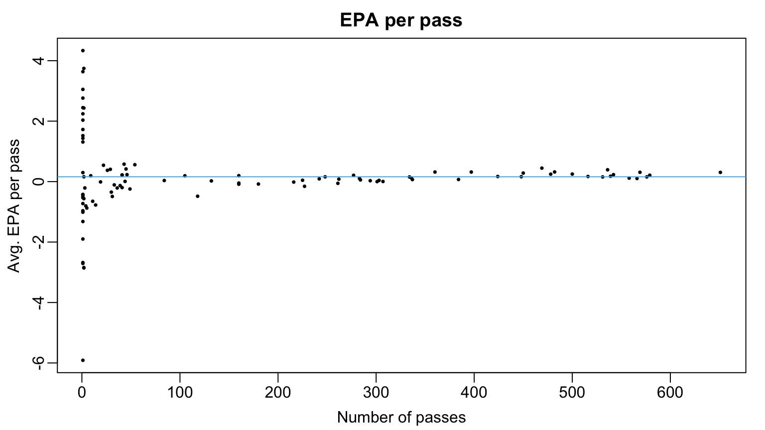
Figure 2: The variability in per-pass decreases dramatically as the number of passes increases.

Thought-Experiment

If $i$ threw many passes, $\hat{\alpha}_{i}$ accurately estimates latent ability $\alpha_{i}$
- Prefer to use $\hat{\alpha}_{i}$ over global mean $\overline{y}$
If $i$ threw very few passes, $\hat{\alpha}_{i}$ can be very noisy
- Global mean $\overline{y}$ arguably better than $\hat{\alpha}_{i}$
What about for players b/w extremes?

Idea: $w_{i} \times \hat{\alpha}_{i} + (1 - w_{i}) \times \overline{y}$
- If $n_{i}$ very large, $w_{i}$ should be closer to 1
- If $n_{i}$ very small, $w_{i}$ should be closer to 0
Problem: how to specify weights in data-driven way?

Multilevel Models

Model Specification

Level 1: observed EPA for player $i$ normally distributed around $\alpha_{i}$
Level 2: Latent player abilities $\alpha_{i}$’s are themselves normally distributed around $\mu$ \[ \begin{align} \textrm{Level 1}&: &\quad Y_{ij} &= \alpha_{i} + \epsilon_{ij}; \epsilon_{ij} \sim N(0, \sigma^{2}) \quad \textrm{for all}\ j = 1, \ldots, n_{i},\ i = 1, \ldots, I \\ \textrm{Level 2}&: &\quad \alpha_{i} &= \alpha_{0} + u_{i}; u_{i} \sim N(0, \sigma^{2}_{\alpha}) \quad \textrm{for all}\ i = 1, \ldots, I \end{align} \]
$\alpha_{0}$: average per-pass EPA over super-population of passers
$\sigma$ captures “within-player” variability in EPA pass-to-pass
$\sigma_{\alpha}$ captures “between-player” variability in per-pass EPA

Level 2 responses $\alpha_{i}$ are not observable
“Borrowing strength”: predition for player $i'$ informed by their data and everyone else’s data
- Estimate of $\alpha_{i}$ informed by $i$’s data **and $\alpha_{0}$
- Estimates of $\alpha_{i}$ determine estimate of $\alpha_{0}$

Hierarchical Structure

Often data exhibits hierarchical grouping structure
- Passes group by QB, players in teams etc.
Grouping variable may be relevant to outcome & induces correlation
Outcomes from same group may be tightly clustered around group average

Fitting Multilevel Models

The (1 | passer_player_id) tells lmer() to include a random intercept for each passer

library(lme4)
multilevel_fit <-
  lmer(formula = epa ~ 1 + (1|passer_player_id), 
       data = pass2024)

Extracting Estimates

Use ranef() to extract estimates $\hat{u}_{i}$’s
Use coef to get $\hat{\alpha}_{i} = \hat{\alpha}_{0} + \hat{u}_{i}$
- Only valid when there is one grouping variable
- W/ more grouping variables, random intercepts not identified
coef() and ranef() return lists w/ one element per grouping variable
- Each list element is a data table

tmp <- coef(multilevel_fit)
tmp[["passer_player_id"]] |> dplyr::slice_head(n = 5)

           (Intercept)
00-0023459  0.11643217
00-0026158  0.14662915
00-0026300  0.12284041
00-0026498  0.16012352
00-0027973  0.01971509

Estimated Random Intercepts $\hat{\alpha}_{i}$

Code
Top & Bottom 5 Passers

Create temporary table lmer_alpha with player name, id, and estimate
Join lmer_alpha to alphas (so we can compare with OLS estimates)

lmer_alpha <- data.frame( 
    lmer = tmp[["passer_player_id"]][,1], 
    gsis_id = rownames(tmp[["passer_player_id"]])) 

alphas <- alphas |>
  dplyr::inner_join(y = lmer_alpha, by = "gsis_id")

                  full_name        lmer   n
1             Lamar Jackson  0.36825428 469
2                Jared Goff  0.33315635 536
3                Josh Allen  0.27342658 482
4                Joe Burrow  0.27172057 651
5            Baker Mayfield  0.27062324 569
6               Andy Dalton  0.01971509 160
7                 Drew Lock  0.01595111 180
8        Anthony Richardson  0.01197563 261
9           Spencer Rattler -0.04081740 227
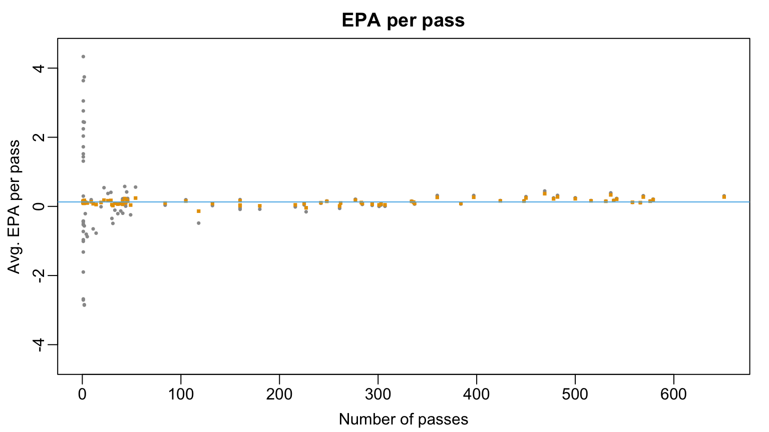
10 Dorian Thompson-Robinson -0.13715503 118

Visualizing Multilevel Estimates

Multilevel model pulls player-specific means to global mean
- Amount of data dictates degree to which original estimate is pulled

Adjusting For Additional Covariates

Simple model doesn’t account for formation, whether QB was hit while throwing, etc.

pass2024 <-
  pbp2024 |>
  dplyr::filter(play_type == "pass" & season_type == "REG") |> 
  dplyr::filter(!grepl("TWO-POINT CONVERSION ATTEMPT", desc) &
                  !grepl("sacked", desc)) |>
  dplyr::select(epa, passer_player_id, 
                air_yards, 
                posteam_type, shotgun, no_huddle, qb_hit,
                pass_location,
                desc) |>
  dplyr::mutate(posteam_type = factor(posteam_type),
                pass_location = factor(pass_location))

Including Fixed Effects

$\boldsymbol{\mathbf{x}}$ contains: air_yards, shotgun, qb_hit, pass_location, posteam_type
Effects of these factors are constant (i.e., fixed) across all passers \[ \begin{align} \textrm{Level 1}&: &\quad Y_{ij} &= \alpha_{i} + \boldsymbol{\mathbf{x}}_{ij}^{\top}\boldsymbol{\beta} + \epsilon_{ij}; \quad \epsilon_{ij} \sim N(0, \sigma^{2}) \\ \textrm{Level 2}&: &\quad \alpha_{i} &= \alpha_{0} + u_{i}; \quad u_{i} \sim N(0, \sigma^{2}_{\alpha}) \end{align} \]

Fitting Our Elaborated Model

ml_fit_full <-
  lme4::lmer(formula = epa ~ 1 + (1|passer_player_id) + 
               air_yards + posteam_type + shotgun +
               no_huddle + qb_hit + pass_location, data = pass2024)

Linear mixed model fit by REML ['lmerMod']
Formula: epa ~ 1 + (1 | passer_player_id) + air_yards + posteam_type +  
    shotgun + no_huddle + qb_hit + pass_location
   Data: pass2024

REML criterion at convergence: 65016.9

Scaled residuals: 
    Min      1Q  Median      3Q     Max 
-8.5225 -0.5478 -0.0841  0.5538  5.4631 

Random effects:
 Groups           Name        Variance Std.Dev.
 passer_player_id (Intercept) 0.01344  0.1159  
 Residual                     2.28043  1.5101  
Number of obs: 17727, groups:  passer_player_id, 103

Fixed effects:
                     Estimate Std. Error t value
(Intercept)          0.133559   0.039314   3.397
air_yards            0.016728   0.001132  14.772
posteam_typehome    -0.010065   0.022883  -0.440
shotgun             -0.109698   0.032192  -3.408
no_huddle            0.021179   0.034703   0.610
qb_hit              -0.470851   0.039760 -11.842
pass_locationmiddle  0.135755   0.030724   4.418
pass_locationright  -0.053875   0.025769  -2.091

Correlation of Fixed Effects:
            (Intr) ar_yrd pstm_t shotgn n_hddl qb_hit pss_lctnm
air_yards   -0.207                                             
postm_typhm -0.280  0.012                                      
shotgun     -0.676 -0.005 -0.011                               
no_huddle   -0.039 -0.009 -0.024 -0.105                        
qb_hit      -0.078 -0.067  0.008  0.005  0.011                 
pss_lctnmdd -0.240 -0.060 -0.013 -0.041 -0.002 -0.019          
pss_lctnrgh -0.348  0.007 -0.010  0.010 -0.003 -0.019  0.441

Top- and Bottom-5 Passers

After adjusting for important fixed effects
- Lamar Jackson has highest EPA/pass
- Dorian Thompson-Robinson had the lowest EPA/pass

                  full_name        lmer
1             Lamar Jackson  0.34106738
2                Jared Goff  0.32096595
3                Joe Burrow  0.29762396
4            Tua Tagovailoa  0.26988653
5                Josh Allen  0.26577678
6              Bailey Zappe  0.03321274
7               Andy Dalton  0.02969282
8        Anthony Richardson -0.01605454
9           Spencer Rattler -0.03511495
10 Dorian Thompson-Robinson -0.08925603

Looking Ahead

EPA is based on starting & ending game state
2 phases of passing play: ball in air + after the catch
Currently analysis implicitly credits QBs for both phases
Lecture 10: divide total EPA among relevant offensive players
Develop a version of WAR
- Multilevel model to estimate per-play contribution
- Scale model estimates by opportunities to create replacement-level shadow

STAT 479 Lecture 9

Motivation

Comparing Football Plays

Play-by-Play Football Data

Player ID

Expected Points

Overivew

Expected Points

Basic Use: Comparing Plays

Basic Uses: Comparing Teams

Predicting EPA on a New Pass

League-Average

Player-Specific Model

Estimating \(\alpha_{i}\)

Small Sample Size

Thought-Experiment

Multilevel Models

Model Specification

Hierarchical Structure

Fitting Multilevel Models

Extracting Estimates

Estimated Random Intercepts \(\hat{\alpha}_{i}\)

Visualizing Multilevel Estimates

Adjusting For Additional Covariates

Including Fixed Effects

Fitting Our Elaborated Model

Top- and Bottom-5 Passers

Looking Ahead