STAT 479: Lecture 8
Defensive Credit & WAR
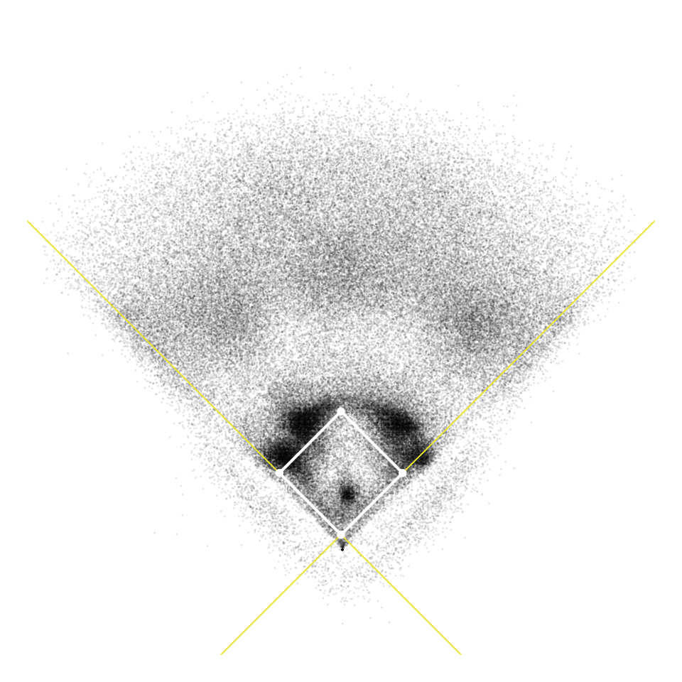
Statcast Coordinates
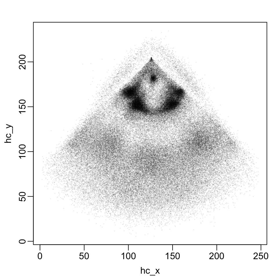
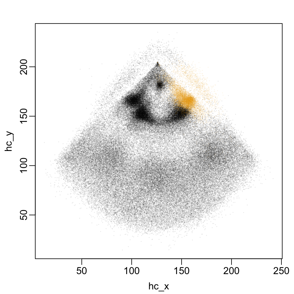
hc_xandhc_y: coordinates where batted ball is first fieldedhit_location: position of player who first fielding ball- Statcast coordinate system
- Home plate at top of plot near
(125, 200) - First baseline on the left
- Units are not in feet
- Home plate at top of plot near
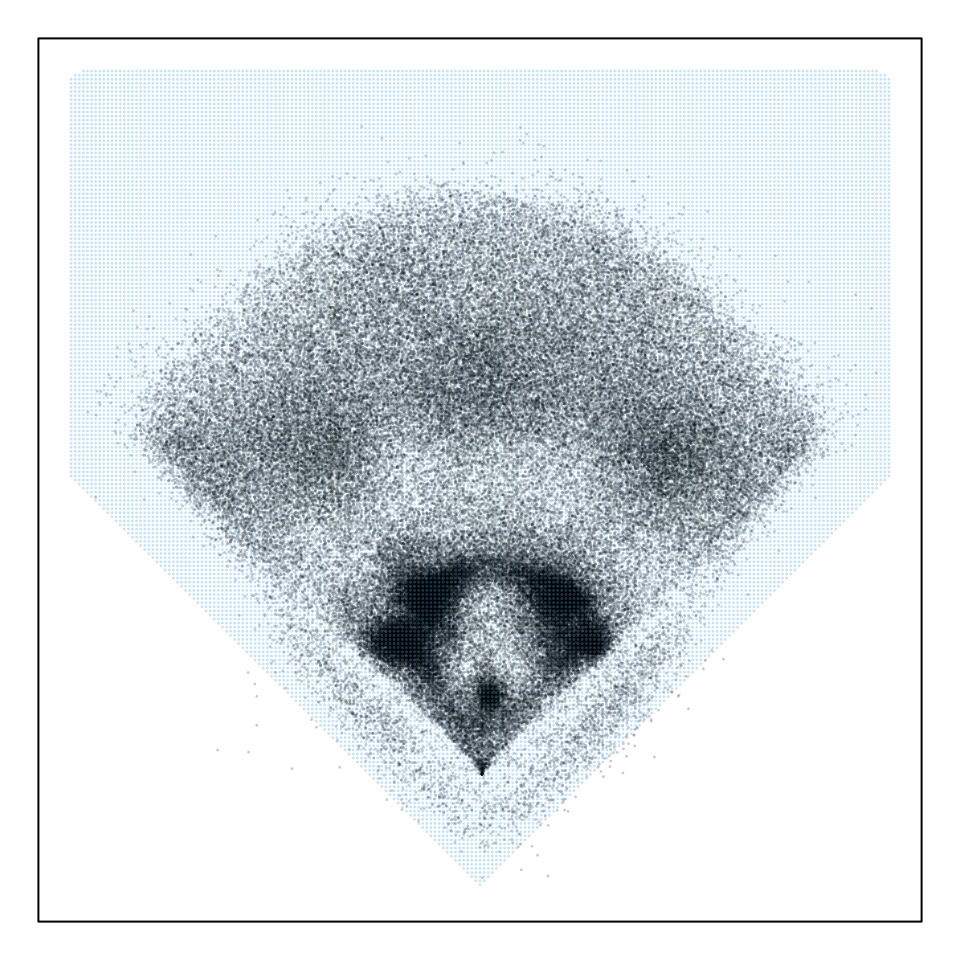
Transformed Coordinates
- Transform:
x = 2.5 * (hc_x - 125.42)&y = 2.5 * (198.27 - hc_y) - Define new coordinate system where
- Home plate at bottom of plot at
(0,0) - Units are in feet
- First base on the right around
(90/sqrt(2), 90/sqrt(2))
- Home plate at bottom of plot at
Binning & Averaging
- Divide field into grid of 3ft x 3ft bins
- Remove unrealistic grid locations
bin_probs <-
  bip |>
  dplyr::select(x, y, Out) |>
  dplyr::mutate(
    x_bin = cut(x, breaks = seq(-300-grid_sep/2, 300+grid_sep/2, by = grid_sep)),
    y_bin = cut(y, breaks = seq(-100 - grid_sep/2, 500+grid_sep/2, by = grid_sep))) |>
  dplyr::group_by(x_bin, y_bin) |>
  dplyr::summarise(
    out_prob = mean(Out),
    n_balls = dplyr::n(),
    .groups = "drop")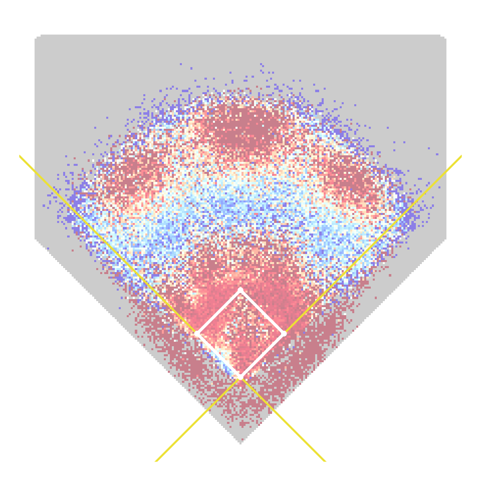
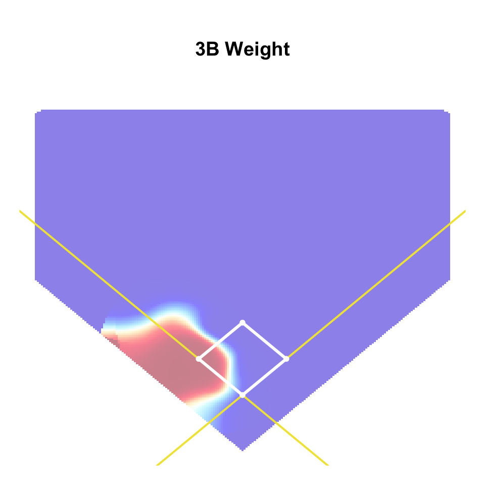
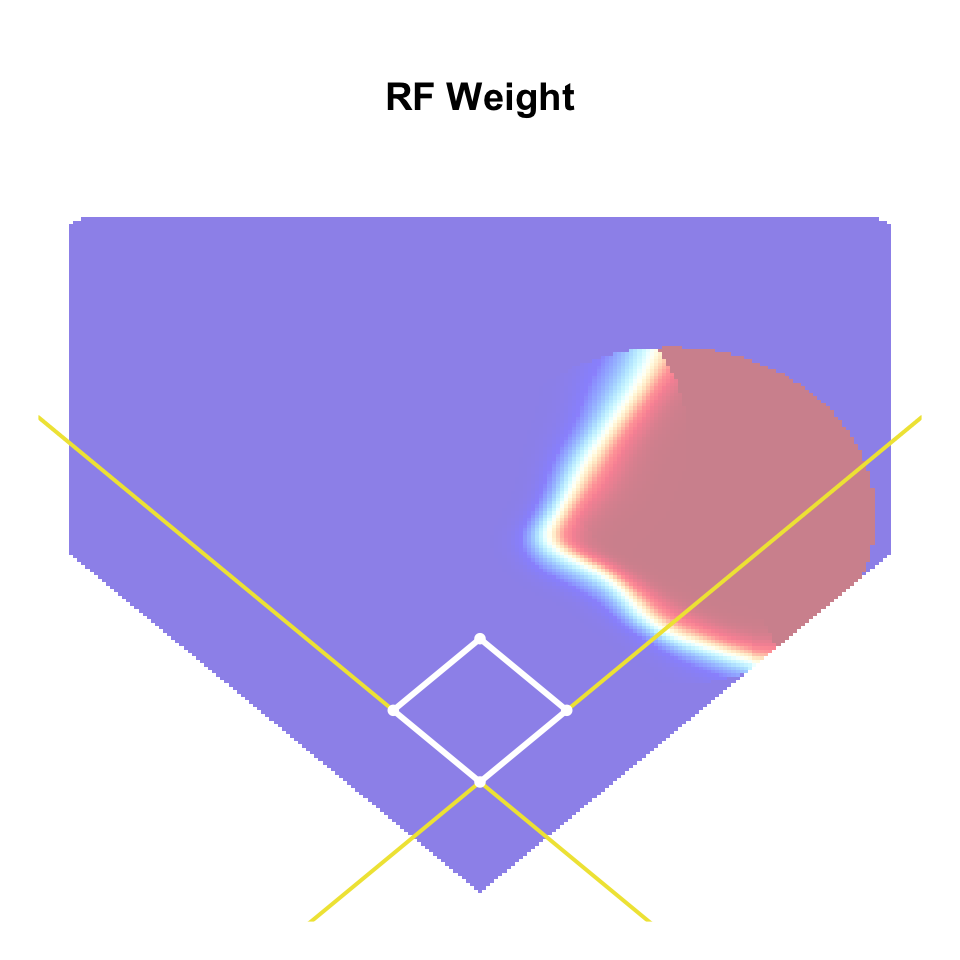
Logistic Regression Estimates

GAM Estimates
- Use
mgcv::bamfor large datasets
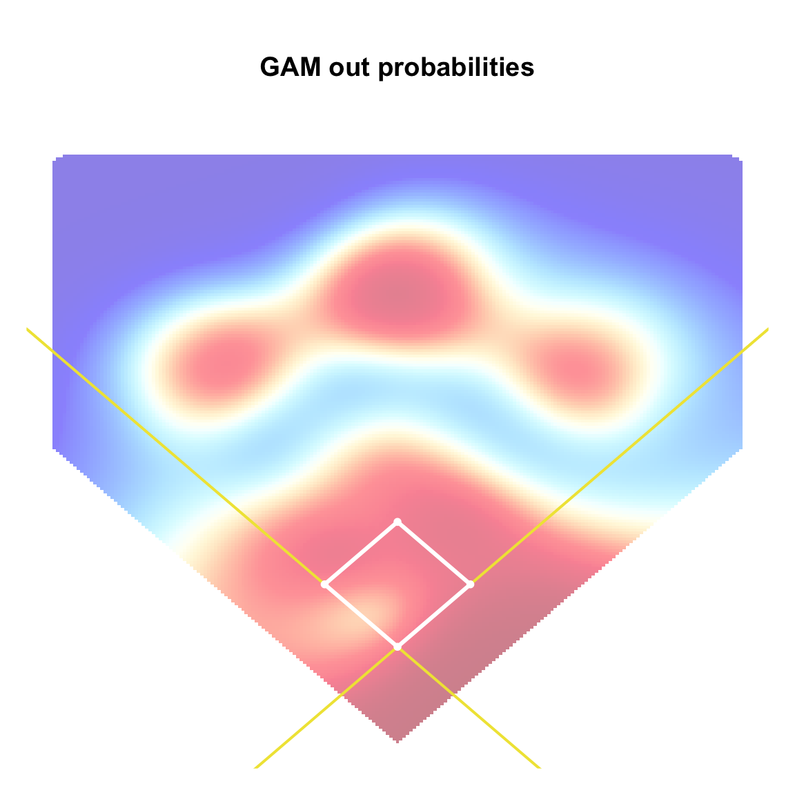
all_preds <-
predict(object = gam_fit,
newdata = def_atbat2024,
type = "response")
def_atbat2024$p_out <- all_preds
def_atbat2024 <-
def_atbat2024 |>
dplyr::mutate(
p_out = dplyr::case_when(
is.na(p_out) & end_events == "home_run" ~ 0,
is.na(p_out) & end_type != "X" ~ 0,
.default = p_out)) |>
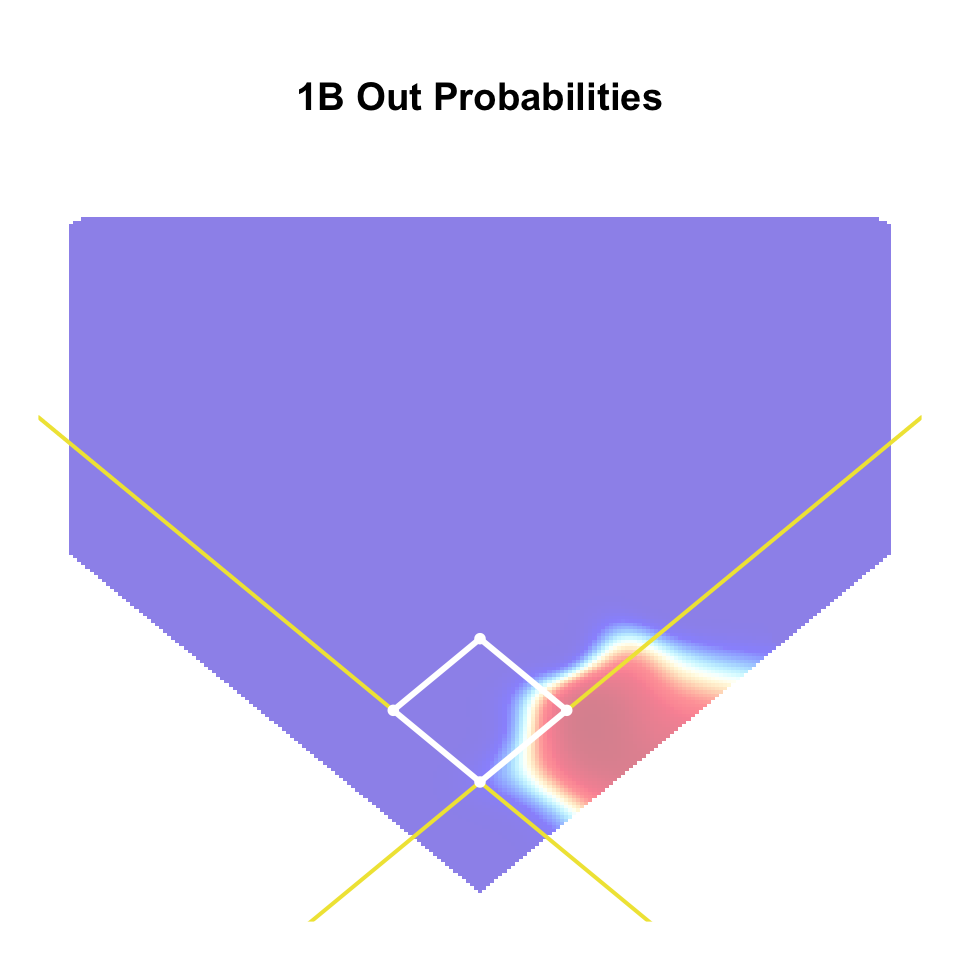
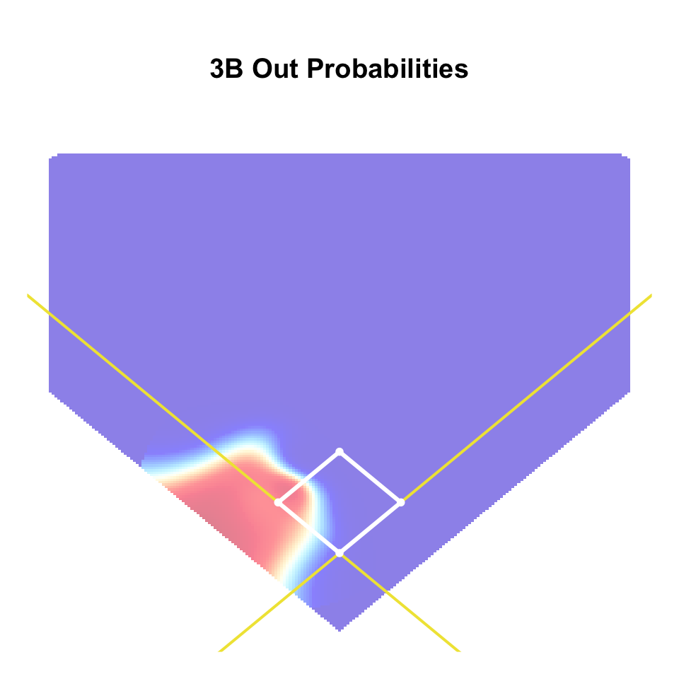
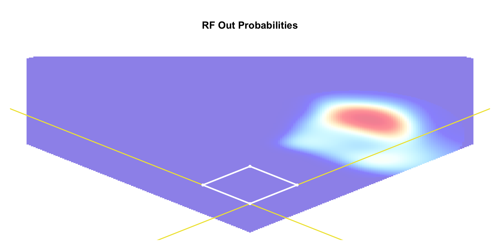
dplyr::filter(!is.na(p_out))Fielder Out Probabilities