STAT 479 Lecture 2

Expected Goals

Motivation & Outline

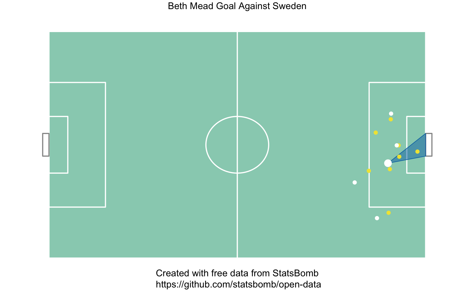
Motivation: Beth Mead in EURO 2022

Beth Mead scored 6 goals in EURO 2022. Which was more impressive?
- Goal in 15th minute against Austria link
- Goal in 37th minute against Norway link
- Goal in 33rd minute against Sweden link

We can argue endlessly about qualitative differences
- One-on-one vs in-traffic; left or right foot;
- Type of shot; time; score; …

Goal: quantitative comparison

A Thought Experiment

What if we could replay each shot over and over again?
How often would she score?

This long-run frequency is Expected Goals (XG)

Soccer Event Data

StatsBomb & Hudl

Player location data for all events
- Computer vision + input from 5 human annotators
- Humans log events (shots, tackles, passes, etc.)
- Computer vision to extra location information
Locations mapped to fixed coordinate system
StatsBombR package: available via GitHub

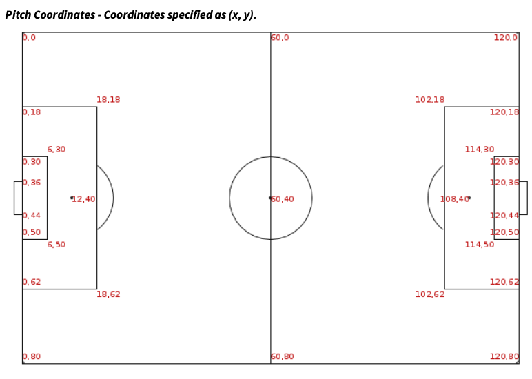
devtools::install_github("statsbomb/StatsBombR")

StatsBomb Coordinates

Offensive action moves left-to-right
Vertical coordinate increases as you move top-to-bottom

Free Competitions

FreeCompetitions() returns table of available competitions

[1] "Whilst we are keen to share data and facilitate research, we also urge you to be responsible with the data. Please credit StatsBomb as your data source when using the data and visit https://statsbomb.com/media-pack/ to obtain our logos for public use."

   competition_id season_id      competition_name season_name
1              16       276      Champions League   1970/1971
2              16        76      Champions League   1999/2000
3               2        44        Premier League   2003/2004
4             116        68 North American League        1977
5              11         1               La Liga   2017/2018
6              43        51        FIFA World Cup        1974
7              53       106     UEFA Women's Euro        2022
8               7       235               Ligue 1   2022/2023
9              11        37               La Liga   2004/2005
10             35        75    UEFA Europa League   1988/1989

Free Matches

StatsBombR::FreeCompetitions() |>
  dplyr::filter(competition_id == 53 & season_id == 106) |> 
  StatsBombR::FreeMatches() |>
  dplyr::select(home_team.home_team_name, away_team.away_team_name, home_score, away_score) |>
  dplyr::slice_sample(n=5)

# A tibble: 5 × 4
  home_team.home_team_name away_team.away_team_name home_score away_score
  <chr>                    <chr>                         <int>      <int>
1 England Women's          Norway Women's                    8          0
2 England Women's          Austria Women's                   1          0
3 Denmark Women's          WNT Finland                       1          0
4 Germany Women's          Austria Women's                   2          0
5 Austria Women's          Norway Women's                    1          0

euro2022_events <-
  StatsBombR::FreeCompetitions() |> 
  dplyr::filter(competition_id == 53 & season_id == 106) |> 
  StatsBombR::FreeMatches() |> 
  StatsBombR::free_allevents() |> 
  StatsBombR::allclean() |> 
  StatsBombR::get.opposingteam()

euro2022_shots <-
  euro2022_events |>
  dplyr::filter(type.name == "Shot" & shot.body_part.name != "Other") |>
  dplyr::mutate(Y = ifelse(shot.outcome.name == "Goal", 1, 0))

 [1] "minute"              "player.name"         "shot.technique.name"
 [4] "shot.body_part.name" "shot.type.name"      "location.x"         
 [7] "location.y"          "DistToGoal"          "DistToKeeper"       
[10] "AngleToGoal"         "AngleToKeeper"       "OpposingTeam"

Mead’s Shots

mead_shots <-
  euro2022_shots |>
  dplyr::filter(player.name == "Bethany Mead")

mead_shots |>
  dplyr::select(OpposingTeam, minute, shot.body_part.name, shot.technique.name, Y)

# A tibble: 15 × 5
   OpposingTeam     minute shot.body_part.name shot.technique.name     Y
   <chr>             <int> <chr>               <chr>               <dbl>
 1 Austria Women's      15 Right Foot          Lob                     1
 2 Norway Women's       29 Right Foot          Normal                  0
 3 Norway Women's       33 Head                Normal                  1
 4 Norway Women's       37 Left Foot           Normal                  1
 5 Norway Women's       52 Right Foot          Volley                  0
 6 Norway Women's       80 Left Foot           Volley                  1
 7 Northern Ireland      5 Head                Normal                  0
 8 Northern Ireland     15 Right Foot          Half Volley             0
 9 Northern Ireland     43 Left Foot           Normal                  1
10 Northern Ireland     56 Right Foot          Normal                  0
11 Northern Ireland     83 Right Foot          Normal                  0
12 Sweden Women's        4 Head                Normal                  0
13 Sweden Women's       19 Left Foot           Normal                  0
14 Sweden Women's       33 Right Foot          Half Volley             1
15 Sweden Women's       46 Left Foot           Normal                  0

Conditional Expectations

Thought Experiment: Repeating Shots

What proportion of repetitions result in goals?
Across all repetitions, conditions kept the same

Setup & Notation

Suppose our data set contains \(n\) shots
For shot \(i = 1, \ldots, n,\) we observe
- \(Y_{i}\): indicator shot resutled in goal (\(Y = 1\)) or not (\(Y = 0\))
- \(\boldsymbol{\mathbf{X}}_{i}\): vector of \(p\) features about the shot
Features could include things like
- Body part used & shot technique
- Dist. to nearest defenders

Conditional Probability

Assumption: data are a representative sample from an infinite super-population of shots
Each shot in super-population characterized by pair \((\boldsymbol{\mathbf{X}}, Y)\)
Repeating shot with features \(\boldsymbol{\mathbf{x}}\) equivalent to sampling from slice of super-population with \(\boldsymbol{\mathbf{X}} = \boldsymbol{\mathbf{x}}.\)

\[ \textrm{XG}(\boldsymbol{\mathbf{x}}) = \mathbb{E}[Y \vert \boldsymbol{\mathbf{X}} = \boldsymbol{\mathbf{x}}] = \mathbb{P}(Y = 1 \vert \boldsymbol{\mathbf{X}} = \boldsymbol{\mathbf{x}}) \]

Two Basic XG Models

Defining The Super-population

Ultimate goal is to assess Mead’s performance in EURO 2022
- Focus on women’s internationals
- Focus on shots attempted w/ foot or head

Get Events
Extract Shots

wi_events <-
  StatsBombR::FreeCompetitions() |> 
  dplyr::filter(competition_gender == "female" & competition_international) |>
  StatsBombR::FreeMatches() |> 
  StatsBombR::free_allevents() |> 
  StatsBombR::allclean() |>
  StatsBombR::get.opposingteam()

wi_shots <-
  wi_events |>
  dplyr::filter(type.name == "Shot" & shot.body_part.name != "Other") |>  
  dplyr::mutate(Y = ifelse(shot.outcome.name == "Goal", 1, 0))

Idealized Calculation

Suppose our only feature is shot.body_part.name


      Head  Left Foot Right Foot 
       920       1280       2560

If we could access infinite super-population, compute \(\textrm{XG}(\text{right-footed shot})\) by
- Forming subgroup containing only right-footed shots
- Calculating proportion of goals score

Practical Calculation

Since we cannot access infinite super-population, we must estimate XG from data
We do so by mimicking idealized calculation
1. Divide data into subgroups based on shot.body_part.name
2. Compute proportion of goals within subgroups
Rely on dplyr’s group_by() functionality to do this

Estimating XG(body part)

xg_model1 <-
  wi_shots |>
  dplyr::group_by(shot.body_part.name) |>
  dplyr::summarise(XG1 = mean(Y), n = dplyr::n())
xg_model1

# A tibble: 3 × 3
  shot.body_part.name   XG1     n
  <chr>               <dbl> <int>
1 Head                0.112   920
2 Left Foot           0.114  1280
3 Right Foot          0.111  2560

Assessing Beth Mead’s Performance

Append XG estimates to mead_shots w/ left_join
Based on bodypart, each goal is about equally impressive

mead_shots <- mead_shots |>
  dplyr::left_join(y = xg_model1 |> dplyr::select(shot.body_part.name, XG1),
                   by = "shot.body_part.name")

# A tibble: 3 × 5
  OpposingTeam    minute shot.body_part.name     Y   XG1
  <chr>            <int> <chr>               <dbl> <dbl>
1 Austria Women's     15 Right Foot              1 0.111
2 Norway Women's      37 Left Foot               1 0.114
3 Sweden Women's      33 Right Foot              1 0.111

Accounting For Shot Technique

Each goal was scored off a different type of shot
What if we condition body part & shot technique?

table(wi_shots |> dplyr::pull(shot.technique.name))


     Backheel Diving Header   Half Volley           Lob        Normal 
           35            10           648            28          3720 
Overhead Kick        Volley 
           17           302

New XG Estimates

XG Estimates
Mead’s Performance

xg_model2 <-
  wi_shots |>
  dplyr::group_by(shot.body_part.name, shot.technique.name) |>
  dplyr::summarize(XG2 = mean(Y), n = dplyr::n(), .groups = "drop")
xg_model2 |> dplyr::arrange(dplyr::desc(XG2))

# A tibble: 14 × 4
   shot.body_part.name shot.technique.name    XG2     n
   <chr>               <chr>                <dbl> <int>
 1 Right Foot          Lob                 0.208     24
 2 Left Foot           Volley              0.163     98
 3 Left Foot           Normal              0.121    947
 4 Right Foot          Normal              0.121   1863
 5 Head                Normal              0.113    910
 6 Right Foot          Backheel            0.103     29
 7 Right Foot          Half Volley         0.0892   426
 8 Right Foot          Overhead Kick       0.0714    14
 9 Left Foot           Half Volley         0.0676   222
10 Right Foot          Volley              0.0637   204
11 Head                Diving Header       0         10
12 Left Foot           Backheel            0          6
13 Left Foot           Lob                 0          4
14 Left Foot           Overhead Kick       0          3

mead_shots <-
  mead_shots |>
  dplyr::inner_join(
    y = xg_model2 |> dplyr::select(-n), 
    by = c("shot.body_part.name", "shot.technique.name"))

mead_shots |>
  dplyr::select(OpposingTeam, minute, shot.body_part.name, shot.technique.name, Y, XG2) |>
  dplyr::slice(c(1, 4, 14))

# A tibble: 3 × 6
  OpposingTeam    minute shot.body_part.name shot.technique.name     Y    XG2
  <chr>            <int> <chr>               <chr>               <dbl>  <dbl>
1 Austria Women's     15 Right Foot          Lob                     1 0.208 
2 Norway Women's      37 Left Foot           Normal                  1 0.121 
3 Sweden Women's      33 Right Foot          Half Volley             1 0.0892

Accounting for more features

Our 2-feature model is still too coarse
- Doesn’t account for distance of shot
- Doesn’t account for defenders and keeper
StatsBomb records many more features about shots

 [1] "shot.type.name"      "shot.technique.name" "shot.body_part.name"
 [4] "DistToGoal"          "DistToKeeper"        "AngleToGoal"        
 [7] "AngleToKeeper"       "AngleDeviation"      "avevelocity"        
[10] "density"             "density.incone"      "distance.ToD1"      
[13] "distance.ToD2"       "AttackersBehindBall" "DefendersBehindBall"
[16] "DefendersInCone"     "InCone.GK"           "DefArea"

How can we adjust for these in our XG model?

Digression: What is the cone?

Cone: area between shot location & goalposts

Idealized Computation

If we could access super-population, easy to condition on more features
- Slice population along \(\mathbf{\boldsymbol{x}}\)
- Compute proportion of goals among the slice with \(\mathbf{\boldsymbol{X}} = \mathbf{\boldsymbol{x}}\)

Can we mimic this with our observed data?

Practical Challenges

Adjust for body part, technique, and # defenders in cone

# A tibble: 10 × 5
   shot.body_part.name shot.technique.name DefendersInCone    XG     n
   <chr>               <chr>                         <dbl> <dbl> <int>
 1 Left Foot           Normal                            7 1         1
 2 Right Foot          Lob                               2 1         1
 3 Right Foot          Normal                           10 1         1
 4 Left Foot           Volley                            0 0.343    35
 5 Right Foot          Overhead Kick                     0 0.333     3
 6 Right Foot          Overhead Kick                     4 0         2
 7 Right Foot          Overhead Kick                     6 0         1
 8 Right Foot          Volley                            5 0        12
 9 Right Foot          Volley                            6 0         9
10 Right Foot          Volley                            7 0         1

Model-based XG

“Binning-and-averaging” not viable w/ many features due to small sample sizes
Statistical models overcome these challenges by “borrowing strength”
\(\textrm{XG}(\boldsymbol{\mathbf{x}})\) informed by shots with \(\boldsymbol{\mathbf{X}} = \boldsymbol{\mathbf{x}}\) and \(\boldsymbol{\mathbf{X}} \approx \boldsymbol{\mathbf{x}}\)
How a model “borrows strength” depends on its underlying assumptions

Several challenges:
- \(\mathbf{\boldsymbol{X}}\) may be high-dimensional
- \(\textrm{XG}\) likely depends on many interactions
- \(\textrm{XG}\) likely highly non-linear
StatsBomb has a proprietary model

StatsBomb’s XG Estimates

shot.statsbomb_xg records proprietary XG estimate
Goal against Sweden had smallest XG and is, therefore, the most impressive

# A tibble: 3 × 5
  OpposingTeam    minute   XG1   XG2 shot.statsbomb_xg
  <chr>            <int> <dbl> <dbl>             <dbl>
1 Austria Women's     15 0.111 0.208             0.361
2 Norway Women's      37 0.114 0.121             0.444
3 Sweden Women's      33 0.111 0.089             0.091

Goals Over Expected

Did Mead Outperform Expectations?

How to interpret the difference \(Y_{i} - \textrm{XG}_{i}\) when it is
- Large & positive
- Large & negative
- Close to 0

Beth Mead scored 2.89 more goals than expected

sum(mead_shots$Y - mead_shots$shot.statsbomb_xg)

[1] 2.896323

Assessing All EURO2022 Players

goe <- 
  euro2022_shots |>
  dplyr::mutate(diff = Y - shot.statsbomb_xg) |>
  dplyr::group_by(player.name) |>
  dplyr::summarise(GOE = sum(diff), Goals = sum(Y), n_shots = dplyr::n()) |>
  dplyr::arrange(dplyr::desc(GOE)) 
goe |> dplyr::slice(c(1:5, (dplyr::n()-4):dplyr::n()))

# A tibble: 10 × 4
   player.name                GOE Goals n_shots
   <chr>                    <dbl> <dbl>   <int>
 1 Alexandra Popp           3.34      6      16
 2 Bethany Mead             2.90      6      15
 3 Alessia Russo            1.79      4      12
 4 Francesca Kirby          1.79      2       5
 5 Lina Magull              1.70      3      14
 6 Ada Stolsmo Hegerberg   -0.829     0       8
 7 Nadia Nadim             -0.886     0       6
 8 Lauren Hemp             -1.26      1      11
 9 Emma Stina Blackstenius -2.15      1      17
10 Wendie Renard           -2.39      0      17

Looking Ahead

I strongly recommend you work through code yourself
- Full code available here
- Try more binning-and-averaging XG estimates w/ other features
- Try to replicate goals over expected with EURO 2025 data
Will post code for plotting all players during a shot
- shot.freeze_frame contains data frame with other players & their positions

Project Groups

Form groups by Friday September 12 (sign up on Canvas)
Use Piazza to help find teammates