STAT 479 Lecture 24

Decathlon Performance

Motivation & Setup

Decathlon Overview

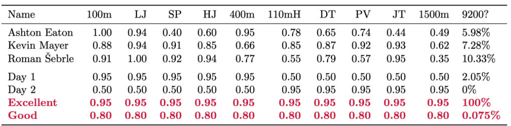
Best Decathlon Performances

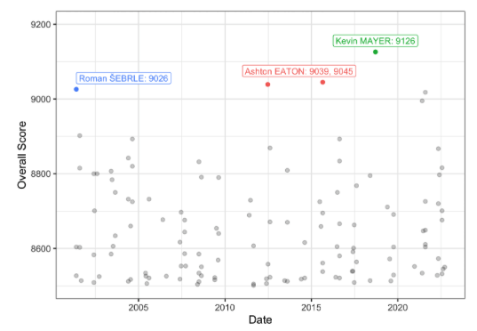
• Can someone break 9200? What would it take?
• Max out in one event? Be good but not elite at all?

Statistical Model

• \(j\)-th performance in event \(e\) by athlete \(i\): \[ \begin{align} y_{e,i,j} &= \alpha_{e,i} + \sum_{d = 1}^{D}{\gamma_{e,d}\phi_{d}(\text{age}_{i,j})} \\ ~& + \beta_{e,1}Y_{1,i,j} + \beta_{e,2}Y_{2,i,j} + \cdots + \beta_{e,e-1}Y_{e-1,i,j} + \epsilon_{e,i,j} \end{align} \]
• Athlete-event random effect: \(\alpha_{e,i} \sim N(\mu_{e}, \sigma_{e})\)
• \(\phi_{d}(x) = x^{d}\): allows for non-linear performance evolution

Model Fitting

• Classical approach: maximum likelihood estimation

  • Find \(\boldsymbol{\alpha}, \boldsymbol{\beta},\) and \(\boldsymbol{\gamma}\) that make observed data most likely
  • Take STAT 310/312/410 for details

• Use \(\boldsymbol{\hat \alpha}, \boldsymbol{\hat \beta},\) and \(\boldsymbol{\hat \gamma}\) to make predictions

• Problem: how to propagate estimation uncertainty to predictions?

Digression: A Bayesian Approach

Types of Uncertainty

• Aleatoric: inherent uncertainty in a system
• Epistemic: due to ignorance/lack of knowledge

• Eg: consider a coin with unknown bias \(\mathbb{P}(\textrm{heads})\)
• Epistemic uncertainty about \(\mathbb{P}(\textrm{heads})\)
  • If we repeatedly flip, we can learn \(\mathbb{P}(\textrm{heads})\)
  • The more data we get, the less uncertainty!
• Aleatoric: uncertainty about result of next flip
  • Even if we know \(\mathbb{P}(\textrm{heads})\), can’t perfectly predict next flip
  • Can’t be reduced!

The Big Bayesian Picture

• Quantify all uncertainties using probability distributions

• Update, combine, and propagate uncertainty using probability calculus

• General workflow: data \(Y\) and unknown parameter \(\theta\)

  • Specify likelihood \(p(y \vert \theta)\) & prior \(p(\theta)\)
  • Compute posterior distribution \(p(\theta \vert y)\)

• Posterior quantifies uncertainty given the observed data

Example: Tea, Milk, Octopi, & FIFA

• Paul the Octopus: predicted football matches
  • Picked from food boxes w/ nations’ flags
  • Correctly predicted \(Y_{1} = 8\) out of 8 games!
• Milk or tea first?
  • Muriel Bristol claimed to taste difference
  • Correctly determined order in \(Y_{2} = 8\) out of 8 cup!

Example: Classical Statistics

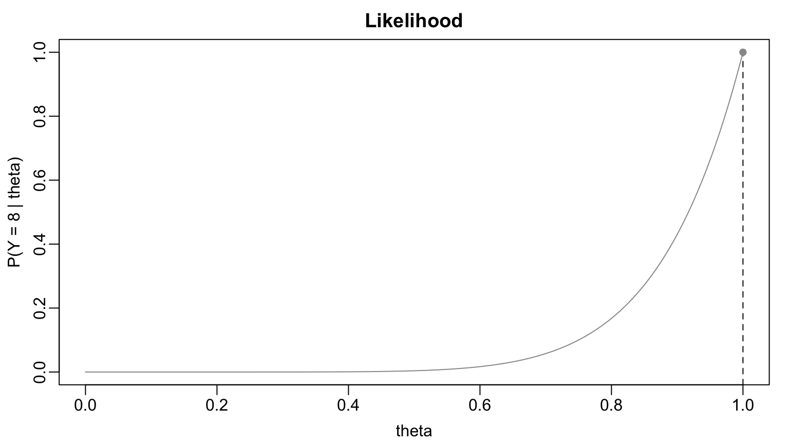
• \(Y_{1} \sim \textrm{Binomial}(8, \theta_{1})\) & \(Y_{2} \sim \textrm{Binomial}(8, \theta_{2}).\)
• We observe \(Y_{1} = Y_{2} = 8\)
• Classical Statistics: \(\hat{\theta}_{1} = \hat{\theta}_{2} = 1\)

Figure 1

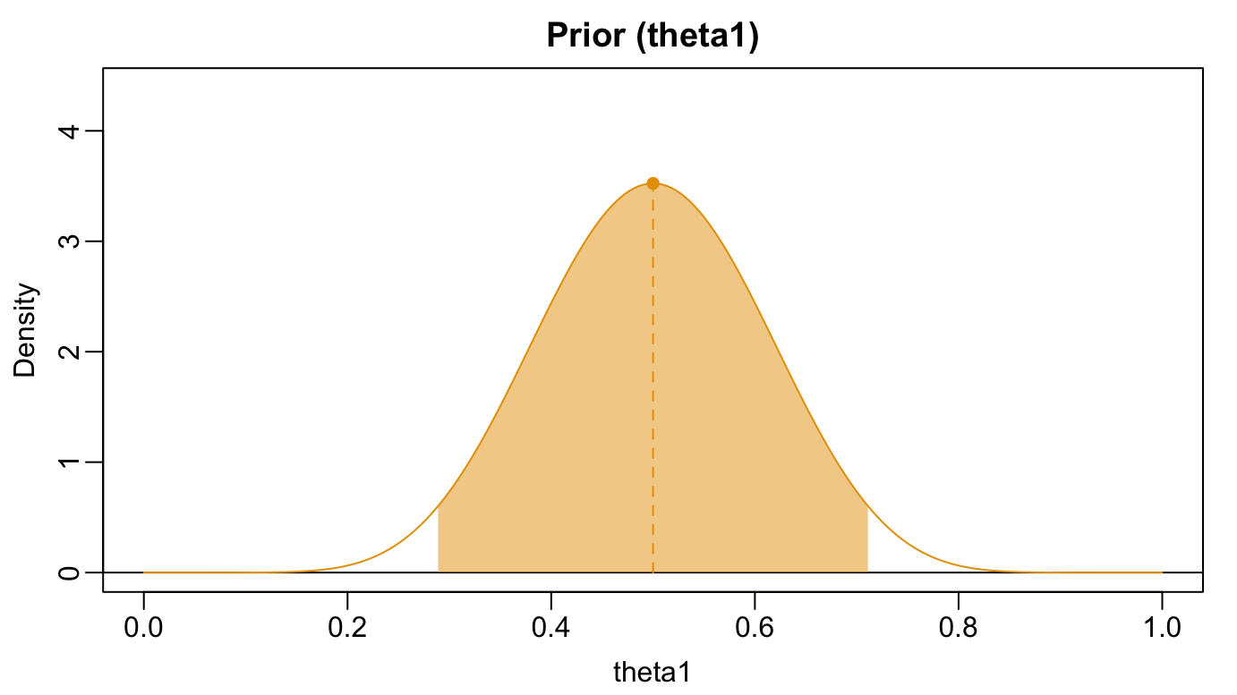
Example: Prior for \(\theta_{1}\)

• Relatively implausible that octopi know soccer
• More likely than not Paul is randomly guessing
• \(\theta_{1} \sim \textrm{Beta}(20,20)\):

Figure 2

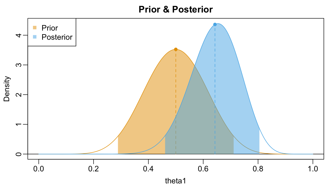
Example: Posterior for \(\theta_{1}\)

• Posterior: \(\theta_{1} \vert Y_{1} = 8 \sim \textrm{Beta}(18, 10)\)
  • Best guess: $_{1} = $ 0.64
  • 95% interval: 0.46, 0.81

Figure 3

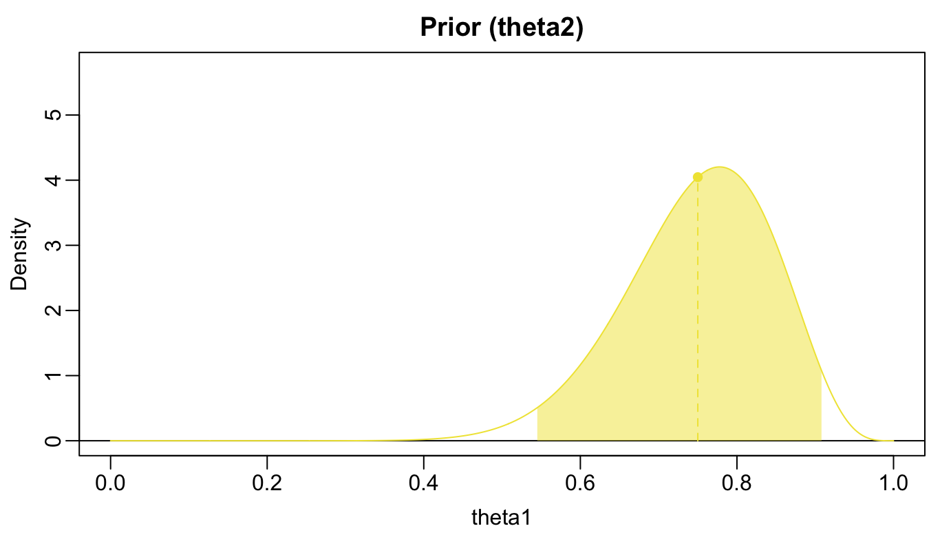
Example: Prior for \(\theta_{2}\)

• Plausible to refine palette over decades of daily tea consumption
• \(\theta_{2}\) is probably over 50%
• \(\theta_{2} \sim \textrm{Beta}(15,5)\)

Figure 4

Example: Posterior for \(\theta_{2}\)

• \(\theta_{2} \vert Y_{2} = 8 \sim \textrm{Beta}(23, 5)\)
  • Best guess: 0.82
  • 95% interval: 0.66, 0.94

Figure 5

Example: Posterior Predictive

• What if we asked Paul & Muriel for 4 more predictions?
• \(\mathbb{P}(Y_{1}^{\star} = k \vert Y_{1} = 8) = \int{ \mathbb{P}(Y_{1}^{\star} = k \vert \theta)p(\theta \vert Y_{1} = 8)d\theta}\)
• Simulation: for \(m = 1, \ldots, M\)
  • Draw a posterior sample \(\theta_{1}^{(m)}\)
  • Then simulate \(Y_{1}^{\star} \sim \textrm{Binomial}(4, \theta_{1}^{(m)})\)

n_sims <- 5e5
theta1_draws <- rbeta(n = 5e5, shape1 = a1_post, shape2 = b1_post)
ystar1 <- rbinom(n = 5e5, size = 4, prob = theta1_draws)
round(table(ystar1)/n_sims, digits = 2)

ystar1
   0    1    2    3    4 
0.02 0.13 0.30 0.36 0.19 

ystar2
   0    1    2    3    4 
0.00 0.03 0.13 0.37 0.48 

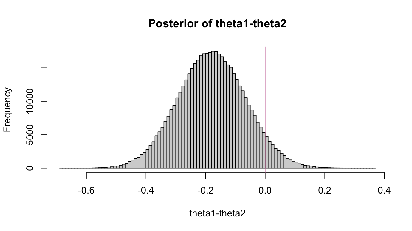
Example: Uncertainty about functionals

• Best estimate for \(\theta_{1} - \theta_{2}\): -0.18; 95% interval -0.4, 0.05
• \(\mathbb{P}(\theta_{1} > \theta_{2} \vert Y_{1} = Y_{2} = 8)\) = 0.06

Figure 6

Advantages of Bayesian Modeling

• Incorporate prior knowledge!
• Multiple parameter values can provide good fits to data
• No longer forced to commit to single estimate to drive downstream prediction
• Can make probabilistic statements: “93% prob. \(\theta\) lies in this interval”
• Sequential nature: use data to update prior beliefs

Bayesian Modeling in Practice

• Most posteriors are not standard distributions
• Must approximate posterior means, quantiles, etc.
• Markov chain Monte Carlo: construct a Markov chain whose invariant dist. is the posterior

Decathlon Modeling Results

Inter-event Dependence

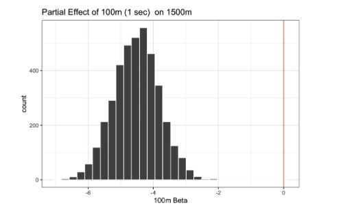
• .1 second decrease in 100m associated w/ ~24 second increase in 1500m time
• Posterior fully concentrated on negative values

Posterior Predictive Simulation

• For each posterior sample \(\boldsymbol{\alpha}^{(m)}, \boldsymbol{\beta}^{(m)}, \boldsymbol{\gamma}^{(m)}, \boldsymbol{\sigma}^{(m)}\): \[ \begin{align} y^{\star(m)}_{e,i,j} &= \alpha^{(m)}_{e,i} + \sum_{d = 1}^{D}{\gamma^{(m)}_{e,d}\phi_{d}(\text{age}_{i,j})} \\ ~& + \beta^{(m)}_{e,1}Y_{1,i,j} + \beta^{(m)}_{e,2}Y_{2,i,j} + \cdots + \beta^{(m)}_{e,e-1}Y_{e-1,i,j} + \sigma^{(m)}\epsilon^{\star (m)}_{e,i,j}, \end{align} \] where \(\epsilon^{\star(m)} \sim N(0,1)\)

• \(y^{\star (1)}_{e,i,j}, \ldots, y^{\star (M)}_{e,i,j}\): sample from posterior of \(Y_{e,i,j}\) given all data.

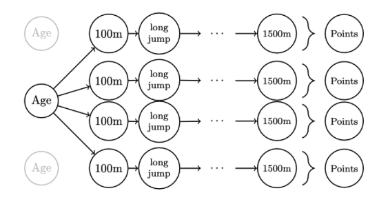
Posterior Predictive Simulations

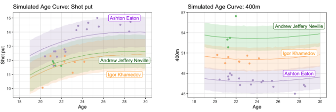
Predicted Age Curve

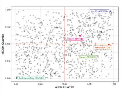
Athlete Profiles

Breaking 9200