STAT 479 Lecture 11

Pitch Framing

Motivation

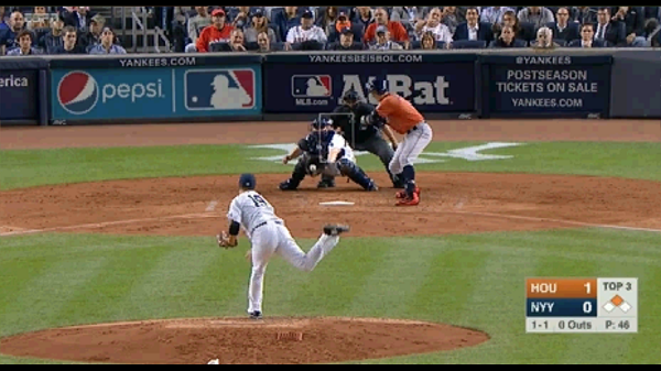
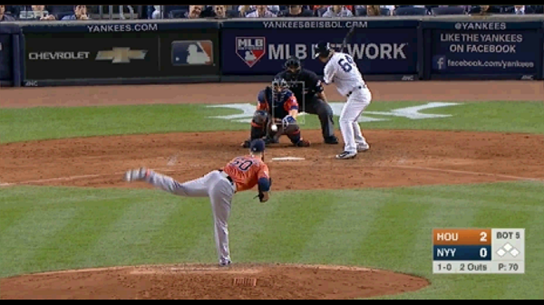
Both pitches miss the strike zone and should, by rule, be called balls
But pitch on the right was called a strike

How much do catchers influence umpires’ calls?

Framing

Ability of catcher to receive pitch so as to increase $\mathbb{P}(\textrm{called strike})$
Ability to “steal a strike” / “turn balls into strikes”
Studied by the sabermetrics community since 2008
Lots of popular press attention b/w 2014 & 2016

Jonathan Lucroy Needs a Raise

According to Baseball Prospectus, Lucroy produced 121 stolen strikes last season and in the past five seasons clocks in at more than 1,000, the most in MLB. And if you believe the metrics, these stolen strikes have been worth about 18 wins during his five-year career – just shy of what Giancarlo Stanton’s entire output has added up to during the same time. Still, Lucroy’s discreetly prodigious output has been underestimated. By fans. By the media. By his own team. And certainly by the game’s salary structure. Even in today’s post-Moneyball world, pitch framing is viewed through a skeptical lens; a value-added talent, sure, but one for which teams are reluctant to pay. While Stanton cashed in with a 13-year, $325 million contract this offseason and Mike Trout begins the first year of his $144.5 million deal, Lucroy was actually more valuable last year. For that he earned $2 million; this year, he’ll make $3 million.

Put another way: The most impactful player in baseball today is the game’s 17th highest-paid catcher.

Overview

Goal: estimate how many runs catcher saves his team
Multilevel model to predict $\mathbb{P}(\textrm{called strike})$
- Random intercepts for batter, pitcher, catcher
- Fixed effect: baseline called strike prob. based on previous season
“Runs Saved Above Replacement”

Value of a Called Strike

Elaborated Run Expectancy

Lectures 6–8: run expectancy at the at-bat level
Today: run expectancy at the pitch level
$\rho(\textrm{o}, \textrm{counts})$:
- Avg. runs scored following pitch in given count & game state
- 3 outs $\times$ 12 counts

Identifying Taken Pitches I

description: pitch-level descriptor

table(statcast2024$description)


                   ball            blocked_ball           bunt_foul_tip 
                 231032                   14717                      15 
          called_strike                    foul               foul_bunt 
                 113912                  126012                    1208 
               foul_tip            hit_by_pitch           hit_into_play 
                   7218                    1979                  121751 
            missed_bunt                pitchout         swinging_strike 
                    196                      52                   73209 
swinging_strike_blocked 
                   3834

Identifying Taken Pitches II

Manually classify description values as called balls or strikes

swing_descriptions <- 
  c("bunt_foul_tip", "foul", "foul_bunt", "foul_tip",
    "hit_into_play", "missed_bunt", "swinging_strike",
    "swinging_strike_block")

taken2024 <- statcast2024 |>
  dplyr::filter(!description %in% swing_descriptions) |> 
  dplyr::mutate(
    Y = ifelse(description == "called_strike", 1, 0), 
    Count = paste(balls, strikes, sep = "-")) |> 
  dplyr::select(
    Y, plate_x, plate_z, Count, Outs,
    batter, pitcher, fielder_2, 
    stand, p_throws, RunsRemaining, sz_top, sz_bot) |> 
  dplyr::mutate(
    Count = factor(Count),
    batter = factor(batter),
    pitcher = factor(pitcher),
    fielder_2 = factor(fielder_2),
    stand = factor(stand),
    p_throws = factor(p_throws))

Pitch-level Run Expectancy

Only use taken pitches in each out-base runner-count state
- er_balls: run expectancy following a called ball in given state
- er_strikes: run expectancy following called strike in given state

Code
Run Expectancy Matrix

er_balls <-
  taken2024 |>
  dplyr::filter(Y == 0) |>
  dplyr::group_by(Count, Outs) |>
  dplyr::summarise(er_ball = mean(RunsRemaining), .groups = 'drop')

er_strikes <-
  taken2024 |>
  dplyr::filter(Y == 1) |>
  dplyr::group_by(Count, Outs) |>
  dplyr::summarise(er_strike = mean(RunsRemaining), .groups = 'drop')

er_taken <-
  er_balls |>
  dplyr::left_join(y = er_strikes, by = c("Count", "Outs")) |>
  dplyr::mutate(value = er_ball - er_strike)

# A tibble: 10 × 5
   Count  Outs er_ball er_strike  value
   <fct> <int>   <dbl>     <dbl>  <dbl>
 1 0-0       0   0.731     0.605 0.126 
 2 0-0       1   0.547     0.425 0.122 
 3 0-0       2   0.283     0.193 0.0902
 4 0-1       0   0.660     0.525 0.135 
 5 0-1       1   0.464     0.365 0.0990
 6 0-1       2   0.234     0.166 0.0684
 7 0-2       0   0.601     0.354 0.247 
 8 0-2       1   0.408     0.211 0.197 
 9 0-2       2   0.163     0     0.163 
10 1-0       0   0.800     0.643 0.157

Most & Least Valuable Called Strikes

For fielding team, a called strike
- In a 3-2 count w/ 0 outs saves 0.8 runs
- In a 0-1 count w/ 2 outs saves 0.07 runs

# A tibble: 4 × 5
  Count  Outs er_ball er_strike  value
  <fct> <int>   <dbl>     <dbl>  <dbl>
1 3-2       0   1.12      0.321 0.800 
2 3-2       1   0.815     0.203 0.612 
3 0-0       2   0.283     0.193 0.0902
4 0-1       2   0.234     0.166 0.0684

Multilevel Modeling

Pitch Location

plate_x and plate_z coordinates of pitch as it cross front of home plate
plate_x measured from catcher’s perspective (right-handed batters stand on the left)

High-Level Model

Level 1: Fixed effects of location ($x$ and $z$) may be non-linear \[ \log \left( \frac{\mathbb{P}(Y_{i} = 1)}{\mathbb{P}(Y_{i} = 0)} \right) = B_{b[i]} + C_{c[i]} + P_{p[i]} + f(x_{i}, z_{i}) \]
Level 2: Random intercepts for Batter, Pither, Catcher \[ \begin{align} B_{i} &= \mu_{B} + u^{(B)}_{b[i]}; u^{(B)}_{b} \sim \mathcal{N}(0,\sigma^{2(B)}) \\ C_{i} &= \mu_{C} + u^{(C)}_{c[i]}; u^{(C)}_{c} \sim \mathcal{N}(0,\sigma^{2(C)}) \\ P_{i} &= \mu_{P} + u^{(P)}_{p[i]}; u^{(P)}_{p} \sim \mathcal{N}(0,\sigma^{2(P)}) \end{align} \]

Idea #1: Assume $f(x,z) = \beta_{X}x + \beta_{Z}z$
- Problem: assumes $\mathbb{P}(\textrm{called strike})$ is monotonic

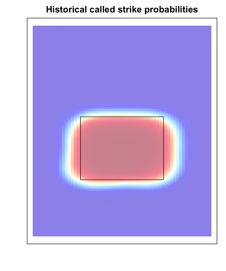
Adjusting for Historical Tendencies

Instead of trying to pre-specify functional form of $f(x,z)$ \[ \log \left( \frac{\mathbb{P}(Y_{i} = 1)}{\mathbb{P}(Y_{i} = 0)} \right) = B_{b[i]} + C_{c[i]} + P_{p[i]} + \beta_{p} \log\left(\frac{\hat{p}(x_{i}, z_{i})}{1 - \hat{p}(x_{i}, z_{i})}\right) \]
$\hat{p}(x,z)$: baseline called strike prob. estimated from 2023 season

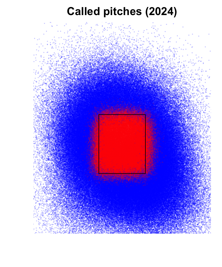
Historical GAM

Filter out pitches too far away from strike zone
- plate_x outside [-1.5, 1.5]
- plate_z outside [1,6]

library(mgcv)
hgam_fit <- 
  bam(formula = Y ~ stand + p_throws + s(plate_x, plate_z),  
      family = binomial(link="logit"), 
      data = taken2023)

Historical Called Strike Probability

Figure 3: Historical called strike probabilities for a right-handed batter facing a right-handed pitcher.

Appending Baseline

Historical GAM trained on 2023 data
Use it to make predictions on all 2024 taken pitches

baseline <- 
  predict(object = hgam_fit,
          newdata = taken2024, 
          type = "link")
taken2024 <-
  taken2024 |>
  dplyr::mutate(baseline = baseline) |>
  dplyr::filter(abs(plate_x) <= 1.5 & plate_z >= 1 & plate_z <= 6)

Fitting our Model

library(lme4)
multilevel_fit <-
  glmer(formula = Y ~ 1 + (1 | fielder_2) + (1 | batter)  + (1 | pitcher) +  baseline, 
        family = binomial(link = "logit"),
        data = taken2024)
summary(multilevel_fit)

Generalized linear mixed model fit by maximum likelihood (Laplace
  Approximation) [glmerMod]
 Family: binomial  ( logit )
Formula: Y ~ 1 + (1 | fielder_2) + (1 | batter) + (1 | pitcher) + baseline
   Data: taken2024

      AIC       BIC    logLik -2*log(L)  df.resid 
 111223.6  111276.3  -55606.8  111213.6    274780 

Scaled residuals: 
    Min      1Q  Median      3Q     Max 
-69.844  -0.135  -0.014   0.116 161.727 

Random effects:
 Groups    Name        Variance Std.Dev.
 pitcher   (Intercept) 0.05122  0.2263  
 batter    (Intercept) 0.02629  0.1621  
 fielder_2 (Intercept) 0.04360  0.2088  
Number of obs: 274785, groups:  pitcher, 851; batter, 649; fielder_2, 100

Fixed effects:
            Estimate Std. Error z value Pr(>|z|)    
(Intercept) 0.084101   0.027122   3.101  0.00193 ** 
baseline    1.027338   0.004563 225.126  < 2e-16 ***
---
Signif. codes:  0 '***' 0.001 '**' 0.01 '*' 0.05 '.' 0.1 ' ' 1

Correlation of Fixed Effects:
         (Intr)
baseline 0.023

Extracting $u^{(C)}_{c}$

Model: $C_{c} = \mu_{C} + u^{(C)}_{c}$ where $u^{(C)}_{c} \sim \mathcal{N}(0,\sigma^{2}_{c})$
Reminder: cannot directly estimate catcher-specific intercepts $C_{c}$ or global average $\mu_{C}$
We can extract deviations $u^{(C)}_{c}$ using ranef()

tmp <- ranef(multilevel_fit)
catcher_u <- 
  data.frame(
    fielder_2 = as.integer(rownames(tmp[["fielder_2"]])),
    catcher_u = tmp[["fielder_2"]][,1])

Runs Saved Above Replacement

Defining Replacement Level

Non-replacement: top $30 \times 2$ catchers sorted by number of pitches caught
$\overline{u}^{(C)}_{R}$: average $u^{(C)}_{c}$ among all replacement-level catchers

catcher_counts <-
  statcast2024 |>
  dplyr::group_by(fielder_2) |>
  dplyr::summarise(count = dplyr::n()) |>
  dplyr::arrange(dplyr::desc(count))

catcher_threshold <- 
  catcher_counts |>
  dplyr::slice(60) |>
  dplyr::pull(count)

catcher_u <-
  catcher_u |>
  dplyr::left_join(y = catcher_counts, by = "fielder_2")

repl_u <-
  catcher_u |>
  dplyr::filter(count < catcher_threshold) |>
  dplyr::pull(catcher_u) |>
  mean()

Counterfactual Predictions

For every taken pitch, use model to predict
- Called strike prob. with original catcher
- Called strike prob. with a replacement-level catcher

Original log-odds:

\[ \mu_{C} + u_{c[i]}^{(C)} + B_{b[i]} + P_{p[i]} + \hat{\beta}_{p} \times \log\left(\frac{\hat{p}(x_{i}, z_{i})}{1 - \hat{p}(x_{i}, z_{i})} \right) \]

Counter-factual log-odds:

\[ \mu_{C} + \overline{u}_{R}^{(C)} + B_{b[i]} + P_{p[i]} + \hat{\beta}_{p} \times \log\left(\frac{\hat{p}(x_{i}, z_{i})}{1 - \hat{p}(x_{i}, z_{i})} \right) \]

ml_preds <-
  predict(object = multilevel_fit,
          newdata = taken2024,
          type = "link")
taken2024 <- taken2024 |>
  dplyr::mutate(fitted_log_odds = ml_preds)

Subtract original $u^{(C)}_{c}$ and add $\overline{u}^{(C)}_{R}$ to log-odds

taken2024 <-
  taken2024 |>
  dplyr::left_join(
    y = catcher_u |> dplyr::select(fielder_2, catcher_u) |>
      dplyr::mutate(fielder_2 = factor(fielder_2)),
    by = "fielder_2") |>
  dplyr::mutate(repl_log_odds = fitted_log_odds - catcher_u + repl_u)

Computing RSAR

Crediting Catcher
Totals
Top-10 RSAR

Weight change in called strike prob. by value of called strike

taken2024 <-
  taken2024 |>
  dplyr::mutate(
    fitted_prob = 1/(1 + exp(-1 * fitted_log_odds)),
    repl_prob = 1/(1 + exp(-1 * repl_log_odds)),
    rsar = value * (fitted_prob - repl_prob))

Sum rsar value across whole season

rsar <-
  taken2024 |>
  dplyr::group_by(fielder_2) |>
  dplyr::summarise(rsar = sum(rsar), n = dplyr::n()) |> 
  dplyr::rename(key_mlbam = fielder_2) |>
  dplyr::left_join(player2024_lookup |>
                     dplyr::select(key_mlbam, Name) |>
                     dplyr::mutate(key_mlbam = factor(key_mlbam)), by = "key_mlbam")

rsar |> 
  dplyr::arrange(dplyr::desc(rsar)) |>
  dplyr::select(Name, rsar) |>
  dplyr::slice_head(n = 10)

# A tibble: 10 × 2
   Name               rsar
   <chr>             <dbl>
 1 Patrick Bailey     29.9
 2 Cal Raleigh        19.8
 3 Austin Wells       17.9
 4 Alejandro Kirk     17.2
 5 Jake Rogers        16.8
 6 Christian Vazquez  15.1
 7 Jose Trevino       14.6
 8 Francisco Alvarez  13.4
 9 Bo Naylor          11.5
10 Yasmani Grandal    11.0

Uncertainty Quantification

Top framers appear to save nearly 30 runs over replacement
Translates to about 3 wins
Exercise: use the bootstrap to quantify uncertainty
- Create several bootstrap re-samples of 2024 taken pitches
- Must re-fit the multilevel model and compute GSAR
- Use the original replacement-level
Quantifying uncertainty: critical to determining monetary value of framing

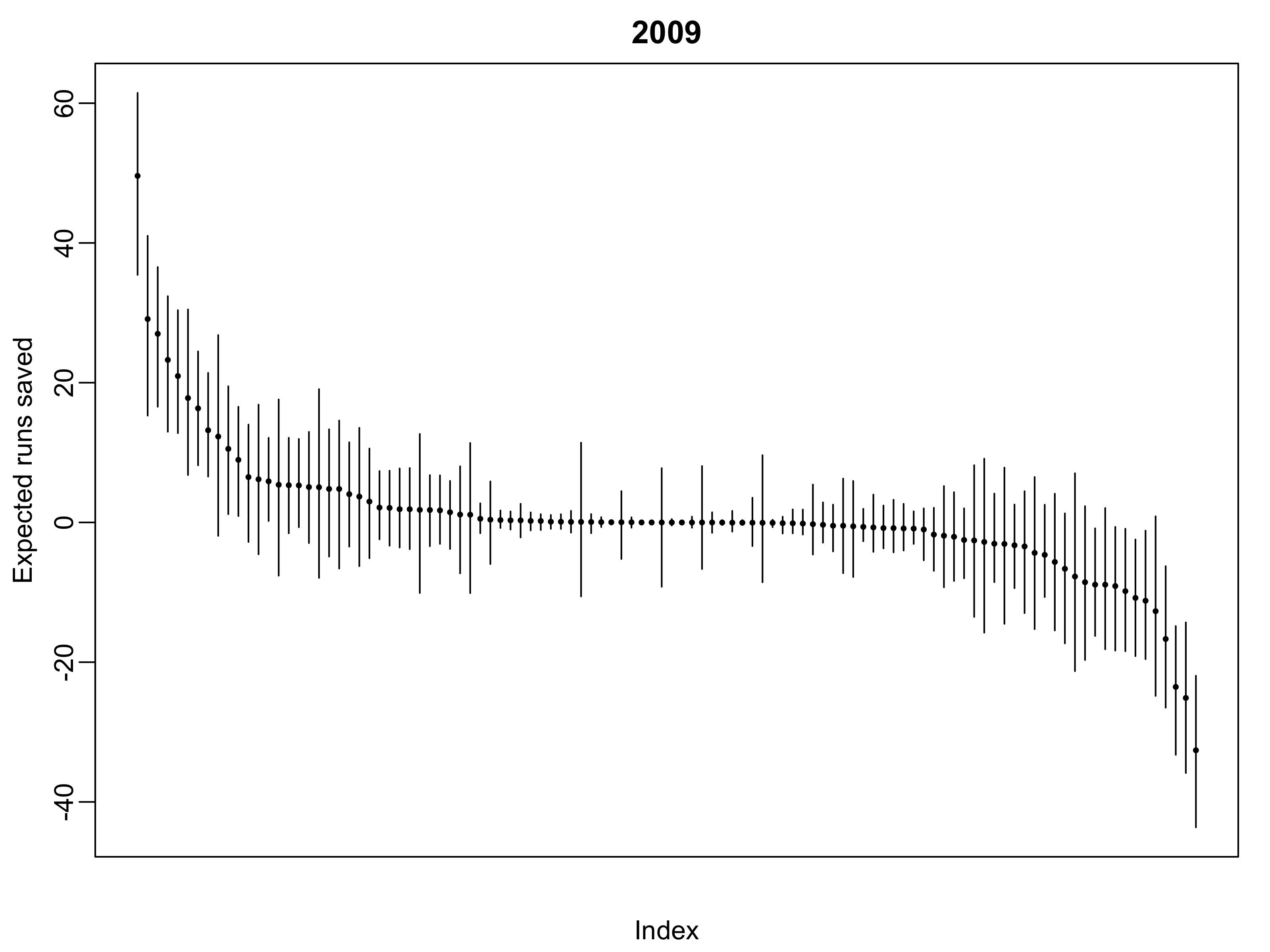
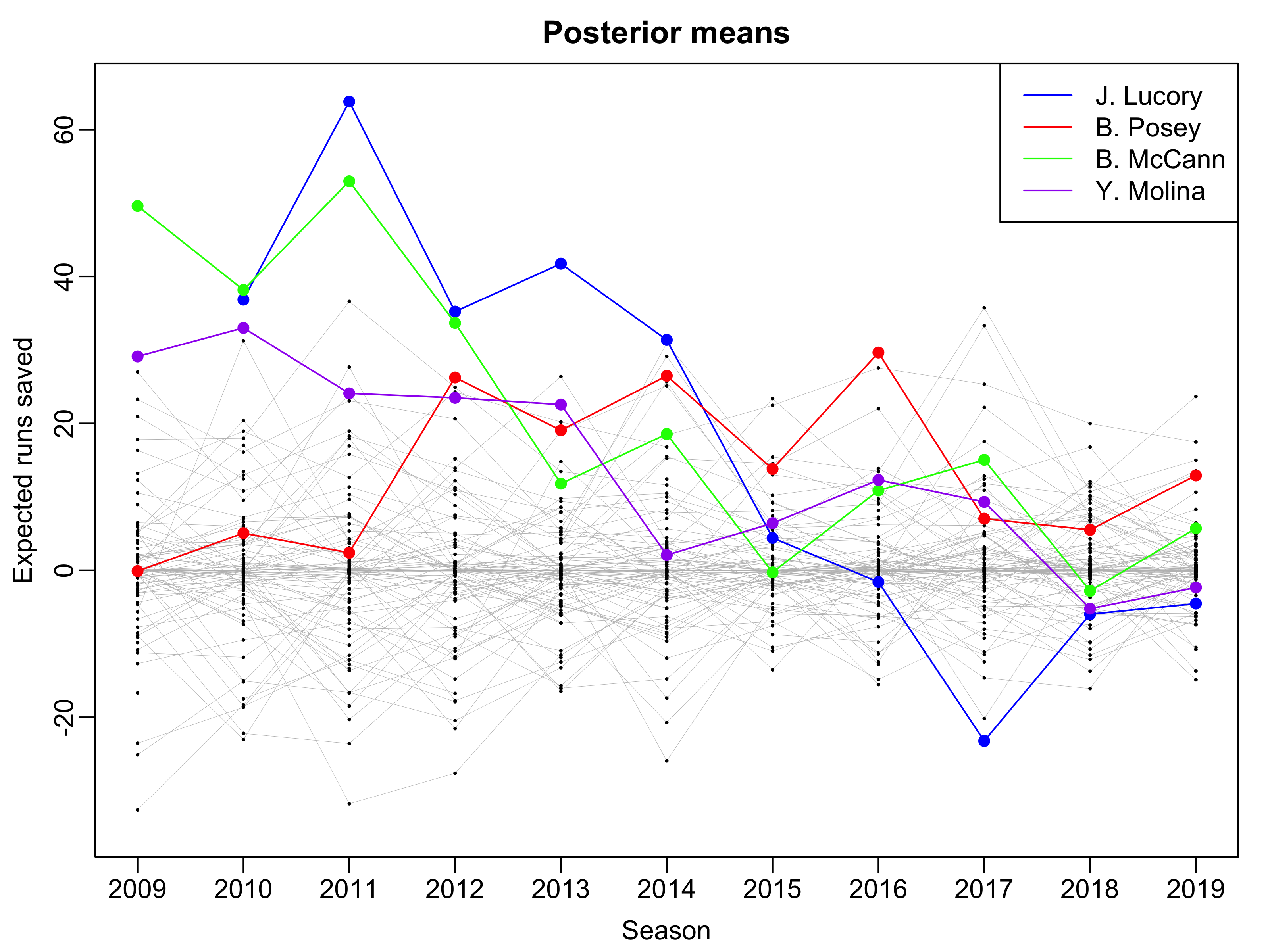
My Own Research

I’ve studied framing since 2015
- Initial paper: Bayesian models to “borrow strength” across umpires
- Conclusion: lots of uncertainty in framing effects
More recently: use Bayesian Additive Regression Trees (BART) to model $\mathbb{P}(\textrm{strike})$
- Faster & more flexible: (2 hours on a desktop vs 50 hours on a cluster)
- Better predictions: mis-classification of 7% vs 10%
- Similar conclusions: possibly large effect but lots of uncertainty

Framing Effectsin 2009

Framing Over Time

Announcements

Projects are due tomorrow at noon
- If you need an extension, email me
- Peer review assignments will be made on Canvas by Sunday night
- Peer review due on Sunday 10/18
Next week: new unit on ranking & simulation
- Lectures 12 & 13: hockey power rankings & the NCAA D1 National Championship
- Lecture 14 & 15: Markov chain simulations
- Lecture 16 & 17: Mock drafts & other simulations
Project 2 Information will be posted by Sunday evening