STAT 479: Lecture 5

Regularized Adjusted Plus/Minus

Recap: Adjusted Plus/Minus

Motivation

How do NBA players help their teams win?
How do we quantify contributions?

Plus/Minus: Easy to compute
- Hard to separate skill from opportunities
- Doesn’t adjust for teammate quality

Adjusted Plus/Minus:
- Regress point differential per 100 possession on signed on-court indicators
- Introduces fairly arbitrary baseline
- Assumes all baseline players have same underlying skill

The Original Model

\(n\): total number of stints
\(p\): total number of players
\(Y_{i}\): point differential per 100 possessions in stint \(i\)

\[ \begin{align} Y_{i} &= \alpha_{0} + \alpha_{h_{1}(i)} + \alpha_{h_{2}(i)} + \alpha_{h_{3}(i)} + \alpha_{h_{4}(i)} + \alpha_{h_{5}(i)} \\ ~&~~~~~~~~~~- \alpha_{a_{1}(i)} - \alpha_{a_{2}(i)} - \alpha_{a_{3}(i)} - \alpha_{a_{4}(i)} - \alpha_{a_{5}(i)} + \epsilon_{i}, \end{align} \]

Matrix Notation

For each stint \(i\) and player \(j\), signed indicator \(x_{ij}\):
- \(x_{ij} = 1\) if player \(j\) on-court at home in stint \(i\)
- \(x_{ij} = -1\) if player \(j\) on-court and away in stint \(i\)
- \(x_{ij} = 0\) if player \(j\) off-court in stint \(i\)

\(\boldsymbol{\mathbf{X}}\): \(n \times p\) matrix of signed indicators
- Rows correspond to stints:
- Columns correspond to players
\(\boldsymbol{\mathbf{Z}}\): \(n \times (p+1)\) matrix
- First column is all ones; remaining are \(\boldsymbol{\mathbf{X}}\)
- \(i\)-th row is \(\boldsymbol{\mathbf{x}}_{i}\)
\(Y_{i} = \boldsymbol{\mathbf{z}}_{i}^{\top}\boldsymbol{\alpha} + \epsilon_{i}\)

Problems w/ Original Model

Individual \(\alpha_{j}\)’s are not statistically identifiable
- E.g. \(\alpha_{j} \rightarrow \alpha_{j}+5\) yields same fit to data
\(\boldsymbol{\mathbf{Z}}\) is not of full-rank
- Can’t invert \(\boldsymbol{\mathbf{Z}}^{\top}\boldsymbol{\mathbf{Z}}\)
Can’t estimate \(\boldsymbol{\alpha}\) with least squares!

A Re-parametrized Model

Assume \(\alpha_{j} = \mu\) for all baseline players \(j\)
For all non-baseline players, \(\beta_{j} = \alpha_{j} - \mu\)
\(\tilde{\boldsymbol{\mathbf{Z}}}\): drop baseline columns from \(\boldsymbol{\mathbf{Z}}\)
\(Y_{i} = \tilde{\boldsymbol{\mathbf{z}}}_{i}^{\top}\boldsymbol{\beta} + \epsilon_{i}\)
Can estimate \(\boldsymbol{\beta}\) with least squares

Problems w/ Re-Parametrized Model

250 minute cut-off for baseline is very arbitrary
Restrictive to assume baseline players have same skill

Baseline assumption needed to use least squares
… but what if we don’t use least squares

Regularized Regression

Ridge Regression

Original APM problem: minimize \(\sum_{i = 1}^{n}{\left(Y_{i} - \boldsymbol{\mathbf{z}}_{i}^{\top}\boldsymbol{\alpha}\right)^{2}}\)

Instead for a fixed \(\lambda > 0\) let’s minimize \(\sum_{i = 1}^{n}{(Y_{i} - \boldsymbol{\mathbf{z}}_{i}^{\top}\boldsymbol{\alpha})^{2}} + \lambda \times \sum_{j = 0}^{p}{\alpha_{j}^{2}},\)

First term: minimized when all \(Y_{i} \approx \boldsymbol{\mathbf{z}}_{i}^{\top}\boldsymbol{\alpha}\)
Second term: shrinkage penalty tries to keep all \(\alpha_{j}\)’s near 0
\(\lambda\): trades-off these two terms

Analytic Solution

For all \(\lambda\), minimizer is \(\hat{\boldsymbol{\alpha}}(\lambda) = \left(\boldsymbol{\mathbf{Z}}^{\top}\boldsymbol{\mathbf{Z}} + \lambda I \right)^{-1}\boldsymbol{\mathbf{Z}}^{\top}\boldsymbol{\mathbf{Y}}.\)
This is almost the OLS solution
- Slightly perturb \(\boldsymbol{\mathbf{Z}}^{\top}\boldsymbol{\mathbf{Z}}\) so it becomes invertible
- E.g., by adding \(\lambda\) to its diagonal

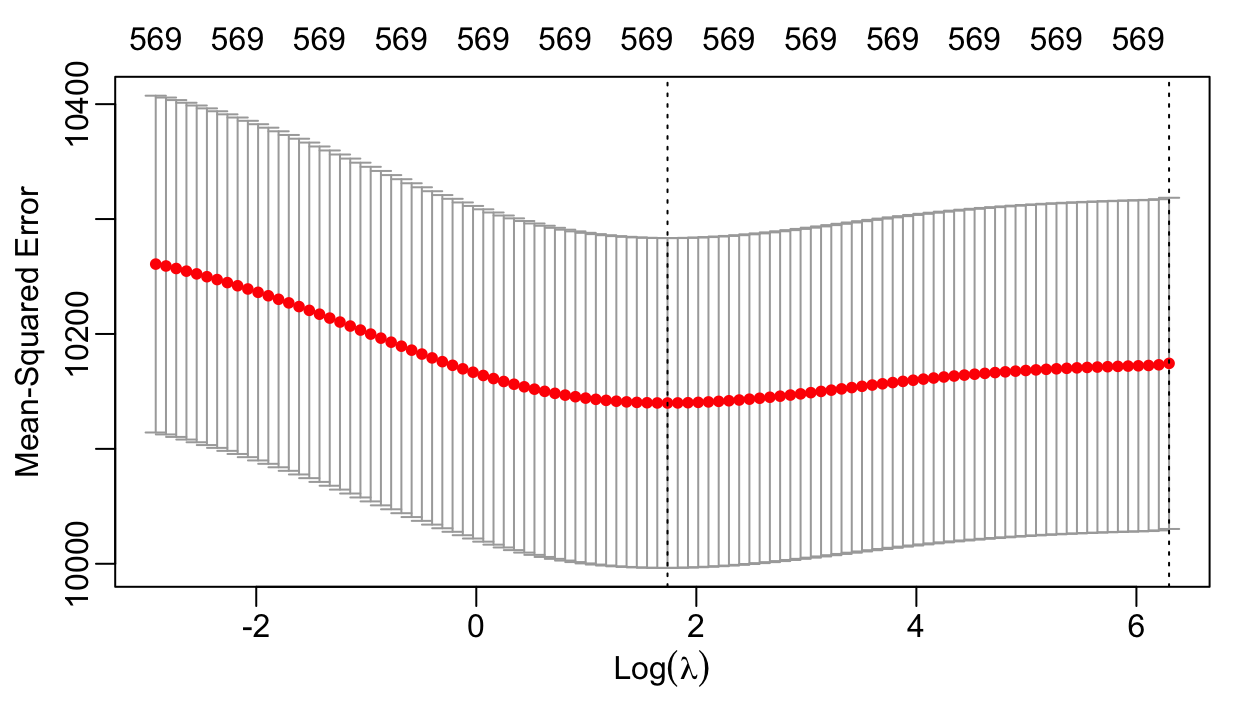
Cross-Validation for \(\lambda\)

Idea: select \(\lambda\) yielding smallest out-of-sample prediction error
Problem: don’t have a separate validation dataset to compute out-of-sample error

Solution: cross-validation to estimate out-of-sample error
- Create a grid of \(\lambda\) values & several train/test splits
  - For each \(\lambda\) and train/test split:
    - Compute \(\hat{\boldsymbol{\alpha}}(\lambda)\) w/ training data
    - Evaluate prediction error using testing data
- For each \(\lambda,\) average testing prediction error across splits
- Identify \(\hat{\lambda}\) w/ smallest average testing error

Compute \(\hat{\boldsymbol{\alpha}}(\hat{\lambda})\) w/ all data

Ridge Regression in Practice

Implemented in the glmnet package
cv.glmnet(): performs cross-validation
- Automatically creates grid of \(\lambda\)
- Default: 10 train/test splits
Important to set standardize = FALSE

set.seed(479) 
library(glmnet) 
cv_fit <-cv.glmnet(x = X_full, y = Y, 
            alpha = 0,
            standardize = FALSE)

Finding \(\hat{\lambda}\)

lambda_min <- cv_fit$lambda.min

Regularized Adjusted Plus/Minus

Extract \(\boldsymbol{\alpha}(\hat{\lambda})\)
Top-10 RAPM
Dončić vs Davis

lambda_index <- which(cv_fit$lambda == lambda_min) 
fit <-glmnet(x = X_full, y = Y, alpha = 0,
         lambda = cv_fit$lambda, 
         standardize = FALSE)

alpha_hat <- fit$beta[,lambda_index]

rapm <- data.frame(id = names(alpha_hat), rapm = alpha_hat) |>
  dplyr::inner_join(y = player_table |> dplyr::select(id,Name), by = "id")

        id     rapm                    Name
1  1628983 3.602143 Shai Gilgeous-Alexander
2  1627827 3.472249     Dorian Finney-Smith
3  1630596 3.415232             Evan Mobley
4  1629029 3.352736             Luka Doncic
5   202699 3.183716           Tobias Harris
6   203999 2.846327            Nikola Jokic
7  1631128 2.829463         Christian Braun
8  1628384 2.813794              OG Anunoby
9   203507 2.646488   Giannis Antetokounmpo
10 1626157 2.641075      Karl-Anthony Towns

Expect to score 3.4 fewer points per 100 possessions with Davis instead of Dončić

luka_rapm <- rapm |> dplyr::filter(Name == "Luka Doncic") |> dplyr::pull(rapm)
ad_rapm <- rapm |> dplyr::filter(Name == "Anthony Davis") |> dplyr::pull(rapm)
ad_rapm - luka_rapm

[1] -3.417006

Other Penalties

For some \(a \in [0,1]\) glmnet() and cv.glmnet() actually minimize \[ \sum_{i = 1}^{n}{(Y_{i} - \boldsymbol{\mathbf{z}}_{i}^{\top}\boldsymbol{\alpha})^{2}} + \lambda \times \sum_{j = 0}^{p}{\left[a \times \lvert\alpha_{j}\rvert + (1-a) \times \alpha_{j}^{2}\right]}, \]
Value of \(a\) specified with alpha argument.
alpha = 0: penalty is \(\sum_{j}{\alpha_{j}^{2}}\)
- Penalty encourage small (but non-zero) \(\alpha_{j}\) values
- Ridge regression; \(\ell_{2}\) or Tikohonov regularization
alpha = 1: penalty is \(\sum_{j}{\lvert \alpha_{j} \rvert}\)
- Penalty encourages sparsity (i.e., sets many \(\alpha_{j} = 0\))
- Least Absolute Shrinkage and Selection Operator (LASSO); \(\ell_{1}\) regularization
\(0 <\)alpha\(<1\): Elastic Net regression

Uncertainty Quantification

The Bootstrap (High-Level Idea)

Say we compute some statistic \(T(\boldsymbol{y})\) using observed data \(\boldsymbol{y}\)
- E.g., RAPM estimate \(\hat{\alpha}_{j}\) for a single player \(j\)
- Estimated difference \(\hat{\alpha}_{j} - \hat{\alpha}_{j'}\) b/w players \(j\) and \(j'\)
- Something more exotic: e.g. \(\max_{j}\hat{\alpha}_{j} - \min_{j}\hat{\alpha_{j}}\)
These are estimates and there is always estimation uncertainty

Repeatedly re-sample data and re-compute statistic
- Re-sampled datasets: \(\boldsymbol{y}^{(1)}, \ldots, \boldsymbol{y}^{(B)}\)
- Corresponding statistics: \(T(\boldsymbol{y}^{(1)}), \ldots, T(\boldsymbol{y}^{(B)})\)
Boostrapped statistics gives a sense of estimate’s variability

Bootstrapping RAPM (plan)

Compute \(\hat{\boldsymbol{\alpha}}(\hat{\lambda})\) using original dataset
Draw \(B\) re-samples of size \(n\)
- Sample observed stints with replacement
For each re-sampled dataset, compute \(\hat{\boldsymbol{\alpha}}(\hat{\lambda})\)
- No need to re-run cross-validation to compute optimal \(\lambda\)
- Use the optimal \(\lambda\) from original dataset
Save the \(B\) bootstrap estimates of \(\boldsymbol{\alpha}\) in an array

set.seed(479)
n <- nrow(X_full)
p <- ncol(X_full)
boot_index <- sample(1:n, size = n, replace = TRUE)

 [1]  1  2  3  4  5  6  6  9 10 11 13 14 14 15 16 17 18 18 19 20

fit <- glmnet(x = X_full[boot_index,], y = Y[boot_index],
              lambda = cv_fit$lambda,
              alpha = 0, standardize = FALSE)

                      Name     Orig Bootstrap
1  Shai Gilgeous-Alexander 3.602143 1.9823702
2      Dorian Finney-Smith 3.472249 1.8454962
3              Evan Mobley 3.415232 3.9265593
4              Luka Doncic 3.352736 2.6188868
5            Tobias Harris 3.183716 2.3872891
6             Nikola Jokic 2.846327 3.1117201
7          Christian Braun 2.829463 2.6171955
8               OG Anunoby 2.813794 1.9276271
9    Giannis Antetokounmpo 2.646488 0.8409495
10      Karl-Anthony Towns 2.641075 4.2211787

Full Bootstrap

B <- 500 
player_names <- colnames(X_full) 
boot_rapm <- matrix(nrow = B, ncol = p, dimnames = list(c(), player_names)) 

for(b in 1:B){
  set.seed(479+b)
  boot_index <- sample(1:n, size = n, replace = TRUE) 
  
  fit <- glmnet(x = X_full[boot_index,], y = Y[boot_index], 
                lambda = cv_fit$lambda,
                alpha = 0,standardize = FALSE)
  tmp_alpha <- fit$beta[,lambda_index]
  boot_rapm[b, names(tmp_alpha)] <- tmp_alpha 
}

Dončić-Davis Contrast

Bootstrap Dist.
Uncertainty Interval

Figure 2: Bootstrap distribution of difference between Doncic & Davis

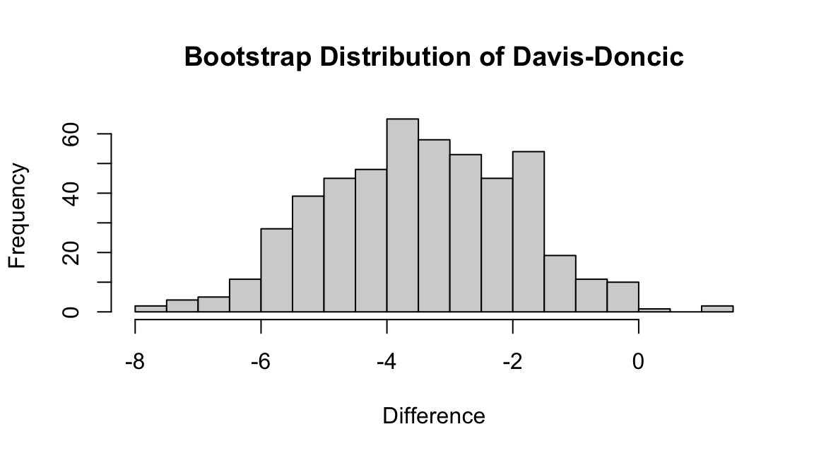
doncic_id <- player_table |> dplyr::filter(Name == "Luka Doncic") |> dplyr::pull(id) 
davis_id <- player_table |> dplyr::filter(Name == "Anthony Davis") |> dplyr::pull(id) 
boot_diff <- boot_rapm[,davis_id] - boot_rapm[,doncic_id]

ci <- quantile(boot_diff, probs = c(0.025, 0.975))
round(ci, digits = 3)

  2.5%  97.5% 
-6.378 -0.484

Visualizing RAPM Uncertainty

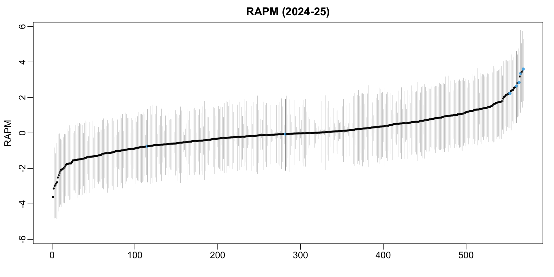
Uncertainty in Ranking

rank() returns sample ranks of vector elements

x <- c(100, -1, 3, 2.5, -2)
rank(x)

[1] 5 2 4 3 1

rank(-1*x)

[1] 1 4 2 3 5

SGA’s RAPM Ranking Uncertainty

Point Estimate
Bootstrapped Ranks
SGA’s Rank

rapm <- rapm |> dplyr::mutate(rank_rapm = rank(-1 * rapm))
rapm |> dplyr::filter(Name == "Shai Gilgeous-Alexander")

       id     rapm                    Name rank_rapm
1 1628983 3.602143 Shai Gilgeous-Alexander         1

MARGIN = 1 applies function to each row

boot_rank <- apply(-1*boot_rapm, MARGIN = 1, FUN = rank)
sga_id <- 
  player_table |> dplyr::filter(Name == "Shai Gilgeous-Alexander") |> dplyr::pull(id)
sga_ranks <- boot_rank[sga_id,]
table(sga_ranks)[1:10]

sga_ranks
 1  2  3  4  5  6  7  8  9 10 
58 59 46 55 36 21 19 12 17 17

SGA had
- Highest RAPM in 58/500 bootstrap re-samples
- 2nd highest RAPM in 59/500 re-samples

Considerable uncertainty in ranks!

quantile(sga_ranks, probs = c(0.025, 0.975))

  2.5%  97.5% 
 1.000 51.525

Looking Ahead

Lectures 6–8: Building up to wins above replacement in baseball
Project Check-in: by Friday 26 September email me a short overview of your project
- Precise problem statement & overview of data and analysis plan
- Happy to help brainstorm & narrow down analysis in Office Hours (or by appt.)
- Inspiration: exercises in lecture notes & project information page

Guest Lecture

Namita Nandakumar (Director of R&D at Seattle Kraken)
“Twitter Is Real Life? Translating Student Research To Team Decision-Making”
Great perspective on how past public-facing projects inform her current team-centric work
6pm on Tuesday 30 September in Morgridge Hall 1524 (this room)