# A tibble: 5 × 7
  stint_id n_pos start_minutes minutes home_points away_points pts_diff
     <dbl> <dbl>         <dbl>   <dbl>       <dbl>       <dbl>    <dbl>
1        1    14          0      5.42           18          12        6
2        2     5          5.42   1.51            2           2        0
3        3     1          6.93   0.220           0           2       -2
4        4     4          7.15   2.17            9           1        8
5 5 13 9.32 4.13 13 11 2STAT 479: Lecture 4
Adjusted Plus/Minus
Motivation
- How do NBA players help their teams win?
- How do we quantify contributions?
- Idea: good players do things that show up in the box score
- Points, rebounds, assists, steals, blocks, turnovers
- Easy to collect, sort, explain
- Fails to account for roles
- 10 assists for a guard vs 10 rebounds by a center
- Problem: should some stats weigh more heavily than others?
- Bigger problem: Not everything appears in the box score
- Setting screens, rotating on defense, communicating
- Good shot selection, diving for loose balls
- The “little things”
Plus/Minus
Definition: Plus/Minus
A player’s plus/minus is the point differential that a player’s team accrues while they are on the court.
Intuition: if your team outscores opponent while you’re on the court, you must be doing something right
To compute, must know who is on the court at all times
Play-by-Play NBA Data
- Entry created when player does something tracked by scorekeeper
- Can use the hoopR package to scrape play-by-play data into R
Stint-Level Data
Stint: period of play b/w substitutions where the same 10 players remain on the court.
Can form a data table from play-by-play log where
- Rows correspond to stints
- Columns for game context: start & end scores, length in minutes, etc.
- Column for every player’s signed on-court indicator
Signed on-court indicators:
- +1 if on-court and playing at home
- -1 if on-court and playing on the road
- 0 if not on court
Data Snapshot
- Context columns:
- Game & Stint ID; num. possessions; duration;
- Start & end scores & times; point differential
- 569 columns of signed on-court indicators
# A tibble: 5 × 7
  stint_id `201143` `201950` `1627759` `1628369` `1628436` `1630202`
     <dbl>    <dbl>    <dbl>     <dbl>     <dbl>     <dbl>     <dbl>
1        1        1        1         1         1         0         0
2        2        1        0         0         1         1         1
3        3        1        0         0         1         1         1
4        4        0        0         0         1         1         1
5        5        0        1         0         1         1         1
player_table <-
hoopR::nba_commonallplayers()[["CommonAllPlayers"]] |>
dplyr::select(PERSON_ID, DISPLAY_FIRST_LAST) |>
dplyr::rename(id = PERSON_ID, FullName = DISPLAY_FIRST_LAST) |>
dplyr::mutate(
Name = stringi::stri_trans_general(FullName, "Latin-ASCII"))
player_table |>
dplyr::filter(id %in% c("201143", "201950", "1627759")) |>
dplyr::pull(FullName)[1] "Jaylen Brown" "Jrue Holiday" "Al Horford" Plus/Minus
Computing Individual +/- (Concept)
Consider Shai Gilgeous-Alexander (2024-25 MVP)
To compute SGA’s +/-:
- Sum the home team point differentials for all stints where SGA was on the court and playing at home.
- Sum the negative of the home team point differentials for all shifts where SGA was on the court and playing on the road.
- Add the two totals from Steps 1 and 2.
Computing Individual +/- (Formula)
- \(\Delta_{i}\): home team point differential in shift \(i\)
- \(x_{i, \textrm{SGA}}\): SGA’s signed on-court indicator:
- \(x_{i, \textrm{SGA}} = 0\) if SGA off-court in stint \(i\)
- \(x_{i, \textrm{SGA}} = 1(-1)\) if SGA on-court at home (away) in stint \(i\)
- SGA’s +/- is just \[ \sum_{i = 1}^{n}{x_{i,\textrm{SGA}} \times \Delta_{i}}. \]
Computing Individual +/- (Code)
- When SGA was on the floor, Thunder outscored opponents by 888 pts
- When Jokic was on the floor, Nuggets outscored opponents by 452
[1] 888Digression: Matrix Computation
Notation
\(n\): total number of stints in the season
\(p\): total number of players
For each stint \(i = 1, \ldots, n\) and player \(j = 1, \ldots, p\):
- \(x_{ij} = 1\) if player \(j\) on-court at home in stint \(i\)
- \(x_{ij} = -1\) if player \(j\) on-court on road in stint \(i\)
- \(x_{ij} = 0\)
\(\Delta_{i}\): home-team differential in stint \(i\) . . .
Player \(j\)’s +/-: \(\sum_{i}{x_{ij}\Delta_{i}}\)
Stint Design Matrix
- Arrange \(x_{ij}\)’s into an \(n \times p\) matrix
\[ \boldsymbol{\mathbf{X}} = \begin{pmatrix} x_{1,1} & \cdots & x_{1,p} \\ \vdots & & \vdots \\ x_{n,1} & \cdots & x_{n,p} \end{pmatrix} \]
- Collect all \(n\) \(\Delta_{i}\)’s into a vector of length \(n\) \[ \boldsymbol{\Delta} = \begin{pmatrix} \Delta_{1} \\ \vdots \\ \Delta_{n} \end{pmatrix} \]
Computing all +/-’s
- Can compute all player’s w/ matrix-vector multiplication \(\boldsymbol{\mathbf{X}}^{\top}\boldsymbol{\Delta}\) \[ \begin{pmatrix} x_{1,1} & \cdots & x_{n,1} \\ \vdots & & \vdots \\ x_{1,p} & \cdots & x_{n,p} \end{pmatrix} \begin{pmatrix} \Delta_{1} \\ \vdots \\ \Delta_{n} \end{pmatrix} = \begin{pmatrix} x_{1,1}\Delta_{1} + x_{2,1}\Delta_{2} + \cdots + x_{n,1}\Delta_{n}\\ \vdots \\ x_{1,p}\Delta_{1} + x_{2,p}\Delta_{2} + \cdots + x_{n,p}\Delta_{n} \end{pmatrix} \]
Computing Plus/Minus
context_vars <-
  c("game_id", "stint_id", "n_pos",
    "start_home_score", "start_away_score", "start_minutes",
    "end_home_score", "end_away_score", "end_minutes",
    "home_points", "away_points", "minutes",
    "pts_diff", "margin")

X_full <- as.matrix(
    rapm_data |> dplyr::select(- tidyr::all_of(context_vars)))
pm <-
data.frame(
id = colnames(X_full),
pm = crossprod(x = X_full, y = rapm_data |> dplyr::pull(pts_diff)),
n_pos = crossprod(abs(X_full), y = rapm_data |> dplyr::pull(n_pos)),
minutes = crossprod(abs(X_full), y = rapm_data |> dplyr::pull(minutes))) |>
dplyr::inner_join(y = player_table |> dplyr::select(id, Name), by = "id") |>
dplyr::select(id, Name, pm, n_pos, minutes) |>
dplyr::arrange(dplyr::desc(pm)) Name pm
1 Shai Gilgeous-Alexander 888
2 Jayson Tatum 474
3 Nikola Jokic 452
4 Giannis Antetokounmpo 331
5 Luka Doncic 276
6 Anthony Davis -78
7 LeBron James -88Visualizing Plus/Minus
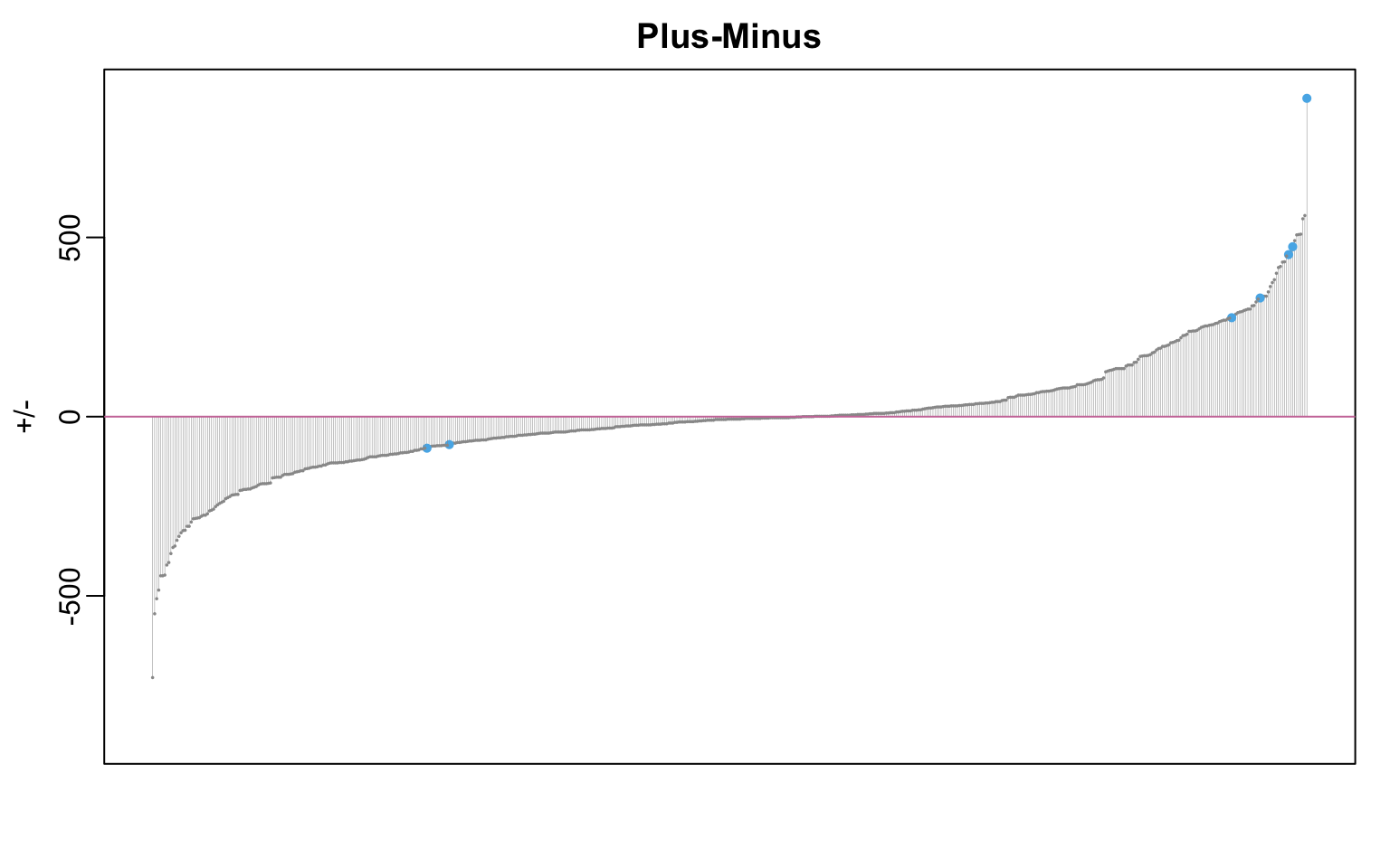
Plus/Minus and Possessions
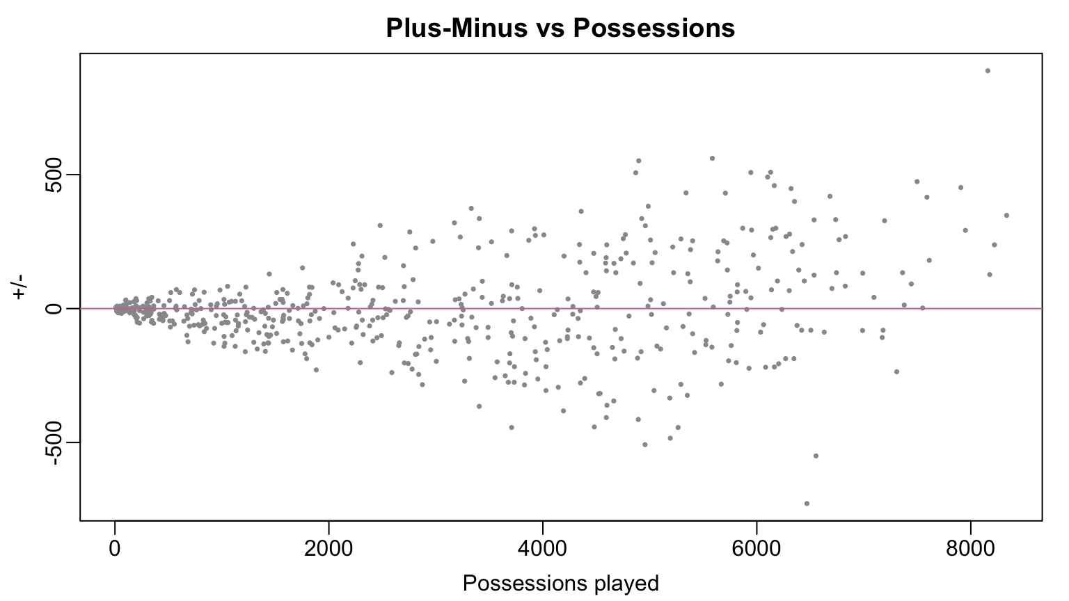
Issues with Plus/Minus
        id                    Name  pm n_pos minutes
1  1628983 Shai Gilgeous-Alexander 888  8159 2837.31
2  1629652           Luguentz Dort 561  5584 1955.17
3  1630198              Isaiah Joe 552  4896 1715.11
4  1628401           Derrick White 509  6129 2327.72
5  1630596             Evan Mobley 508  5944 2049.43
6  1630598           Aaron Wiggins 507  4868 1683.08
7  1628378        Donovan Mitchell 491  6101 2106.53
8  1628369            Jayson Tatum 474  7498 2840.95
9  1628386           Jarrett Allen 459  6163 2142.82
10 203999 Nikola Jokic 452 7907 2707.97- Is Lou Dort really better than Jayson Tatum???
- Differences in +/- could be a result of
- Differences in skill
- Differences in playing time
- Differences in teammate & opponent quality
Adjusted Plus/Minus
From Totals to Rates
- Comparing totals favors players with more playing time
- APM works with rates: point differential per 100 possessions
# A tibble: 10 × 4
   stint_id pts_diff n_pos margin
      <dbl>    <dbl> <dbl>  <dbl>
 1        1        6    14   42.9
 2        2        0     5    0
 3        3       -2     1 -200
 4        4        8     4  200
 5        5        2    13   15.4
 6        6        4     8   50
 7        8        6     9   66.7
 8        9        5    29   17.2
 9       10        0     6    0
10       11       -2     5  -40
An Initial APM Model
- Associate each player \(j\) with a latent strength \(\alpha_{j}\)
- \(\alpha_{j}\)’s are unknown: they must be estimated from data
- \(Y_{i}\): point differential per 100 possessions in stint \(i\)
- \(h_{1}(i), \ldots, h_{5}(i)\) & \(a_{1}(i), \ldots, a_{5}(i)\): identities of players on court in stint \(i\)
\[ \begin{align} Y_{i} &= \alpha_{0} + \alpha_{h_{1}(i)} + \alpha_{h_{2}(i)} + \alpha_{h_{3}(i)} + \alpha_{h_{4}(i)} + \alpha_{h_{5}(i)} \\ ~&~~~~~~~~~~- \alpha_{a_{1}(i)} - \alpha_{a_{2}(i)} - \alpha_{a_{3}(i)} - \alpha_{a_{4}(i)} - \alpha_{a_{5}(i)} + \epsilon_{i}, \end{align} \]
Example
- Dec 23, 2024 game Dallas Mavericks (away) at Golden State Warriors (home):
- DAL: Luka Doncic, Dereck Lively II, Kyrie Irving, P.J. Washington, and Klay Thompson
- GSW: Stephen Curry, Buddy Hield, Andrew Wiggins, Jonathan Kuminga, and Kevon Looney.
- Per 100 possessions, with these lineups DAL expects to outscore GSW by \[ -1 \times (\alpha_{0} + \alpha_{SC} + \alpha_{BH} + \alpha_{AW} + \alpha_{JK} + \alpha_{KL}) +(\alpha_{LD} + \alpha_{KI} + \alpha_{DL} + \alpha_{PW} + \alpha_{KT}). \]
- Now imagine that you replaced Doncic w/ Anthony Davis.
- Per 100 possessions, DAL expects to outscore GSW by \[ -1 \times (\alpha_{0} + \alpha_{SC} + \alpha_{BH} + \alpha_{AW} + \alpha_{JK} + \alpha_{KL}) +(\alpha_{AD} + \alpha_{KI} + \alpha_{DL} + \alpha_{PW} + \alpha_{KT}). \]
- DAL expects to score \(\alpha_{\textrm{AD}} - \alpha_{\textrm{LD}}\) more points per 100 possessions with Davis than Doncic, all else being equal
Potential Issue: Interpretation
- Individual \(\alpha_{j}\)’s are meaningless!
- \(\alpha_{j}\): change in point differential per 100 possessions b/w
- Playing 5-on-5 w/ player \(j\) on the court
- Playing 5-on-4 w/ player \(j\) off the court
- Luckily, we can interpret differences (or contrasts) like \(\alpha_{j}-\alpha_{j'}\)
APM As A Linear Model
- Append a column of 1’s to \(\boldsymbol{\mathbf{X}}\) to form \(n \times (p+1)\) matrix \(\boldsymbol{\mathbf{Z}}\)
- Let \(\boldsymbol{\mathbf{z}}_{i}\) be the \(i\)-th row of \(\boldsymbol{\mathbf{Z}}\)
- APM asserts: \(Y_{i} = \boldsymbol{\mathbf{z}}_{i}^{\top}\boldsymbol{\alpha} + \epsilon_{i}.\)
- Tempting to estimate \(\boldsymbol{\alpha}\) with least squares \[ \textrm{argmin} \sum_{i = 1}^{n}{\left( Y_{i} - \boldsymbol{\mathbf{z}}_{i}^{\top}\boldsymbol{\alpha} \right)^{2}} . \]
Non-identifiability
- Recall that the model asserts \[ \begin{align} Y_{i} &= \alpha_{0} + \alpha_{h_{1}(i)} + \alpha_{h_{2}(i)} + \alpha_{h_{3}(i)} + \alpha_{h_{4}(i)} + \alpha_{h_{5}(i)} \\ ~&~~~~~~~~~~- \alpha_{a_{1}(i)} - \alpha_{a_{2}(i)} - \alpha_{a_{3}(i)} - \alpha_{a_{4}(i)} - \alpha_{a_{5}(i)} + \epsilon_{i}, \end{align} \]
- Imagine we add 5 to every \(\alpha_{j}\): right-hand side remains unchanged
- While we can’t hope to learn \(\alpha_{j}\)’s exactly, can still interpret constrasts \(\alpha_{j} - \alpha_{j'}\)
Singularity
- Least squares problem does not have a unique solution!
- Columns of \(\boldsymbol{\mathbf{Z}}\) are linearly dependent
- The first element in each row is equal to 1 (for intercept)
- 5 entries equal to 1 (for home players)
- 5 entries equal to -1 (for away players)
- If you know all but one column, you can perfectly determine that column
- \(\boldsymbol{\mathbf{Z}}^{\top}\boldsymbol{\mathbf{Z}}\) not invertible
Baseline Contrasts
- Classify certain players as “baseline”-level (e.g., \(< 250\) minutes)
- Re-number players so first \(p'\) are non-baseline
- Assumption: \(\alpha_{j} = \mu\) for all baseline players \(j > p'\)
- All baseline players assumed to have the same underlying skill
- For non-baseline \(j = 1, \ldots, p,\) let \(\beta_{j} = \alpha_{j} - \mu\)
- \(\beta_{j}\): effect of replacing player \(j\) with a baseline player
A Re-parametrized Model
- \(\tilde{\boldsymbol{\mathbf{Z}}}\) be the \(n \times (p'+1)\) submatrix of \(\boldsymbol{\mathbf{Z}}\) s.t.
- First column is all 1’s
- Remaining columns: signed on-court indicators for non-baseline players
- Turns out:
- \(\tilde{\boldsymbol{\mathbf{Z}}}\boldsymbol{\beta} = \boldsymbol{\mathbf{Z}}\boldsymbol{\alpha}\)
- There quantity \(\sum_{i = 1}^{n}{\left(Y_{i} - \tilde{\boldsymbol{\mathbf{z}}}_{i}^{\top}\boldsymbol{\beta}\right)^{2}}\) has a unique minimizer
\[ \hat{\boldsymbol{\beta}} = \left( \tilde{\boldsymbol{\mathbf{Z}}}^{\top}\tilde{\boldsymbol{\mathbf{Z}}}\right)^{-1}\tilde{\boldsymbol{\mathbf{Z}}}^{\top}\boldsymbol{\mathbf{Y}}. \]
Estimating \(\boldsymbol{\beta}\)
                    Name      apm
1          Tobias Harris 17.01331
2         Mouhamed Gueye 16.79320
3           Devin Carter 16.60148
4             Trae Young 15.13287
5  Giannis Antetokounmpo 14.61082
6            Isaiah Wong 14.50091
7           Nikola Jokic 14.40837
8         Alperen Sengun 13.55544
9        Quenton Jackson 13.13962
10    Karl-Anthony Towns 13.13714
Weighted Adjusted Plus/Minus
Missing Context
- APM does not account for context
- Can over-inflate garbage-time performance when outcome essentially determined
“can artificially can artificially inflate the importance of performance in low-leverage situations, when the outcome of the game is essentially decided, while simultaneously deflating the importance of high-leverage performance, when the final outcome is still in question. For instance, point differential-based metrics model the home team’s lead dropping from 5 points to 0 points in the last minute of the first half in exactly the same way that they model the home team’s lead dropping from 30 points to 25 points in the last minute of the second half”.
A Weighted Version of APM
- Introduce weight \(w_{i}\) for stint \(i\)
- Find \(\tilde{\boldsymbol{\beta}}\) minimizing \(\sum{w_{i}\left(Y_{i} - \tilde{\boldsymbol{\mathbf{z}}}_{i}^{\top}\boldsymbol{\beta}\right)^{2}}\)
- Solution: letting \(\boldsymbol{\mathbf{W}}\) denote diagonal matrix w/ entries \(w_{i}\) \[ \hat{\boldsymbol{\beta}}_{w} = \left( \tilde{\boldsymbol{\mathbf{Z}}}^{\top}\tilde{\boldsymbol{\mathbf{Z}}}\right)^{-1}\tilde{\boldsymbol{\mathbf{Z}}}^{\top}\boldsymbol{\mathbf{W}}\boldsymbol{\mathbf{Y}} \]
Estimating wAPM
- Example weights:
- \(w_{i} = 1\) if lead \(< 10\)
- \(w_{i} = 0\) if one team leads by \(> 30\) at start of \(i\)
- \(w_{i} = 1 - (\textrm{StartDiff} - 10)/20\): if \(10 \leq \textrm{lead} \leq 30\)
                Name     wapm
1       Devin Carter 19.48318
2      Tobias Harris 17.11044
3    Lauri Markkanen 15.20344
4     Mouhamed Gueye 14.76474
5         Trae Young 14.52393
6       Nikola Jokic 14.14573
7     Alperen Sengun 14.03023
8         OG Anunoby 13.96219
9  Jordan McLaughlin 13.73760
10      Jericho Sims 13.27850
Looking Ahead
- (w)APM is quite sensitive to certain choices:
- Definition of baseline players
- Choice of weights
- Constant baseline skill assumption is highly unsatisfactory
- Issues due to inability to use least squares
- Next time: alternative estimation strategy
- Avoids having to specify baseline players
- Estimates a latent strength for all players
Project 1
- Thanks for sorting yourselves into group!
- If you still don’t have a group, let me know!
- On Canvas, you need to be in a group under “Projects 1&2 Groups”
- Project information posted:
- Requirements for written report and presentation
- Non-exhaustive list of project topics
- Main requirement: must use play-by-play or event-level data
- I.e., use data more granular than game- or season-level totals
- Project Check-in: by Friday 26 September email me a short overview of your project
- Precise problem statement & overview of data and analysis plan
- Happy to help brainstorm & narrow down analysis in Office Hours (or by appt.)