Fitting heteroskedastic models with flexBART

Overview

flexBART now supports fitting heteroskedastic models with Bayesian ensembles of regression trees. Specifically, it can be used to fit models of the form \[ Y \sim \mathcal{N}(\mu(x), \sigma(x)^2) \] where both \(\mu(X)\) and \(v(x)\) are approximated with an ensemble of regression trees. flexBART allows the size (specified using the optional argument M_vec or M), the tree prior hyperparameters (specified using the optional arguments alpha_vec and beta_vec), and the variables used for splitting (specified via the formula argument) to vary in each ensemble.

Example

We first demonstrate flexBART’s functionality using data generated from the model \(Y \sim \mathcal{N}(\mu(x), \sigma(x)^2)\) where \(X\) contains a single continuous covariate.

We generate \(n = 1000\) training observations and \(n = 101\) testing observations.

set.seed(727)
n_train <- 1000
n_test <- 101
n_tot <- n_train + n_test

X = runif(n_tot)
X[(n_train + 1):n_tot] <- seq(0, 1, by = 0.01) # set the test points so we can plot the estimated function
Z = rnorm(n_tot)
mu = 4 * X^2
sigma = 0.2 * exp(2 * X)
Y = mu + sigma * Z

df = data.frame(Y, X)
train_data = df[1:n_train,]
test_data = data.frame(X = df[-c(1:n_train), colnames(df) != "Y"])

We’re now ready to fit our model.

set.seed(101)
fit = flexBART::flexBART(Y ~ bart(.) + sigma(.),
                         train_data = train_data,
                         test_data = test_data
                         )

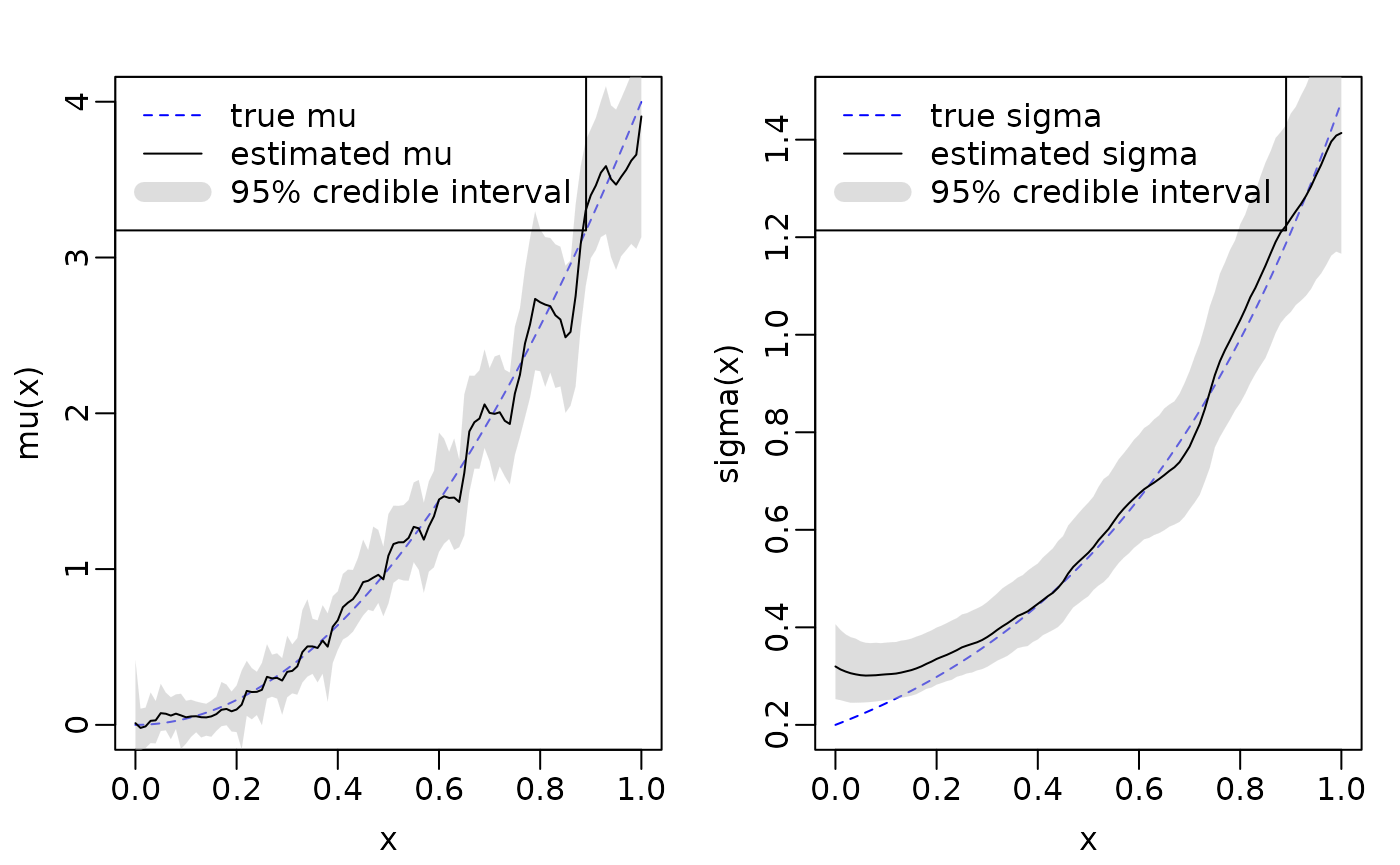
flexBART::flexBART returns the posterior mean estimate and posterior samples for \(\mu(x)\) (outputs named yhat) and \(\sigma(x)\) (outputs named sigma). We plot the true underlying \(\mu(x)\) and \(\sigma(x)\) functions along with the mean and 95% credible intervals estimated by flexBART::flexBART.

mu_l95 <- apply(fit$yhat.test, MARGIN = 2, FUN = quantile, probs = 0.025)
mu_u95 <- apply(fit$yhat.test, MARGIN = 2, FUN = quantile, probs = 0.975)

sigma_l95 <- apply(fit$sigma.test, MARGIN = 2, FUN = quantile, probs = 0.025)
sigma_u95 <- apply(fit$sigma.test, MARGIN = 2, FUN = quantile, probs = 0.975)

par(mar = c(3,3,2,1), mgp = c(1.8, 0.5, 0), mfrow = c(1,2))

plot(0, type = "n", xlim = c(0, 1), ylim = range(mu), xlab = "x", ylab = "mu(x)")
lines(test_data$X, mu[-c(1:n_train)], lty = "dashed", col = "blue")
polygon(x = c(test_data$X, rev(test_data$X)), y = c(mu_l95, rev(mu_u95)), col = scales::alpha("grey", alpha = 0.5), border = FALSE)
lines(test_data$X, fit$yhat.test.mean)
legend("topleft", legend = c("true mu", "estimated mu", "95% credible interval"), col = c("blue", "black", scales::alpha("grey", alpha = 0.5)), lty = c("dashed", "solid", "solid"), lwd = c(1, 1, 10))

plot(0, type = "n", xlim = c(0, 1), ylim = range(sigma), xlab = "x", ylab = "sigma(x)")
lines(test_data$X, sigma[-c(1:n_train)], lty = "dashed", col = "blue")
polygon(x = c(test_data$X, rev(test_data$X)), y = c(sigma_l95, rev(sigma_u95)), col = scales::alpha("grey", alpha = 0.5), border = FALSE)
lines(test_data$X, fit$sigma.test.mean)
legend("topleft", legend = c("true sigma", "estimated sigma", "95% credible interval"), col = c("blue", "black", scales::alpha("grey", alpha = 0.5)), lty = c("dashed", "solid", "solid"), lwd = c(1, 1, 10))